

A contract clause asks for an MTBF of 100 hours. Three suppliers deliver, each system runs a thousand hours of trials, and each records ten failures. Ten failures in a thousand hours is an MTBF of 100 hours, three times over. Every supplier has met the clause.
The first system failed nine times inside its first fifty hours and then settled down. The second failed at a steady drip, roughly once every hundred hours, all the way through. The third ran untroubled for most of the trial and then failed ten times in quick succession near the end. Those are three completely different products, heading for three completely different support contracts, and the number in the clause cannot tell them apart.
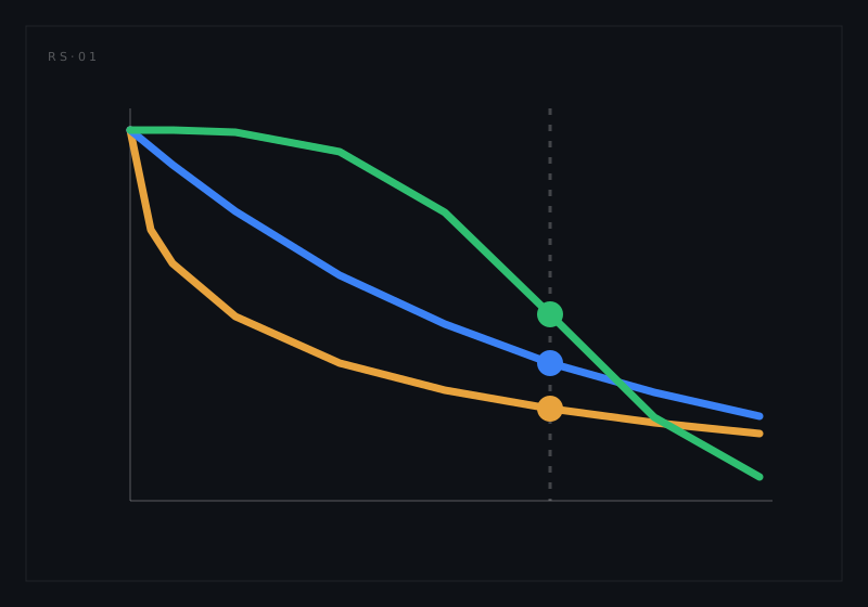
Three systems, one number
Start with the arithmetic, because none of it is in dispute. MTBF for a repairable system is total operating time divided by the number of failures. A thousand hours and ten failures gives a hundred hours, whatever the pattern of arrivals. Nothing has been computed incorrectly anywhere.
What the number cannot express is when the failures arrived, and when is the whole of the engineering question. The first system has a manufacturing or screening problem: units leave the factory carrying defects that surface immediately. The second is behaving like a mature design in its useful life, failing at a steady rate for reasons that are effectively random. The third has a wear-out mechanism, something consuming a finite life, and it reached the end of that life during the trial.
Customers experience these as three unrelated products. The first ruins an entry into service and then behaves itself. The second needs a spares pipeline and a repair loop, indefinitely. The third looks superb right up to a fleet-wide cliff that arrives at roughly the same age for every unit, which is the worst of the three to meet unprepared.
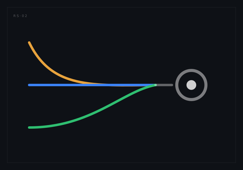
What an average throws away
MTBF is a first moment, the mean of a distribution. Two distributions can share a mean and share almost nothing else, and it is the shape, not the mean, that carries the engineering.
Put numbers on it. Model each system as a population of units whose time to failure follows a Weibull distribution, all three with a mean life of 100 hours, differing only in shape parameter: 0.5 for the early-failure system, 1.0 for the steady one, 3.5 for the wear-out one.
At 50 hours, half the mean life, the fraction of units still running is 37 per cent, 61 per cent and 94 per cent respectively.
The time by which one unit in ten has failed, the B10 life, is under an hour for the first system, about ten hours for the second, and about sixty hours for the third. Two orders of magnitude of difference between products with identical MTBF.
By 150 hours the ranking has inverted: 18 per cent, 22 per cent and 6 per cent are still running. The system that looked best at the halfway mark is the worst by the end. No single number could have carried any of that.
The exponential assumption hiding inside the number
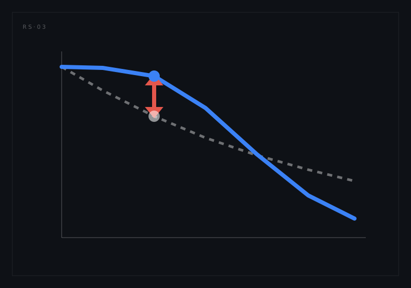
The formula everyone reaches for is R(t) = exp(-t / MTBF), and it is worth being precise about when it holds: only when the hazard rate is constant, which is to say only for the middle system.
Even there it surprises people. Set t equal to the MTBF and the survival probability is 36.8 per cent, not 50. A system operated for exactly its mean time between failures is more likely than not to have failed already. That single fact retires a good deal of casual optimism about big MTBF figures.
Applied to the other two systems the formula is not merely wrong; it is wrong in a direction that changes with the physics. At 50 hours it predicts 61 per cent survival. The wear-out system actually has 94 per cent, so the shortcut libels a good design. The early-failure system actually has 37 per cent, so the same shortcut flatters a bad one. An error that flips sign depending on the failure mechanism cannot be treated as a margin.
There is a related habit worth breaking in the same breath. MTBF is not service life. An MTBF of 100,000 hours does not promise that a unit lasts eleven years. It describes a rate of failure during useful life, and says nothing whatever about when wear-out begins.
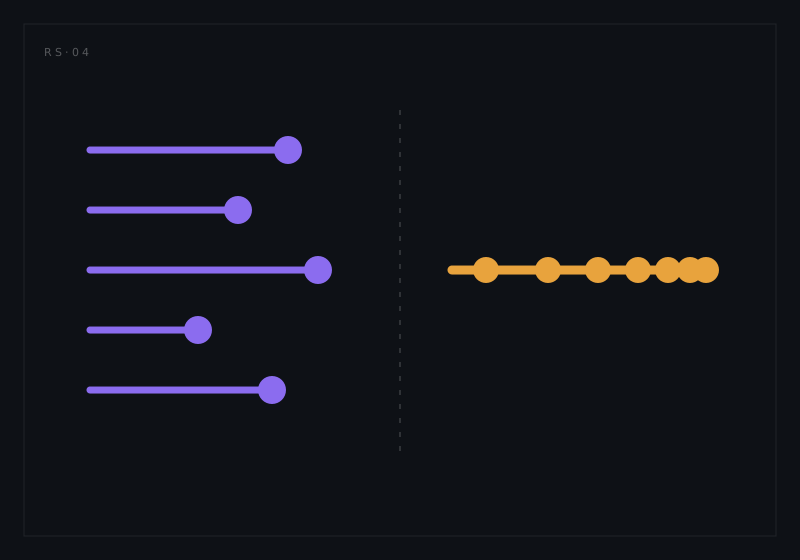
The same Greek letter, two different models
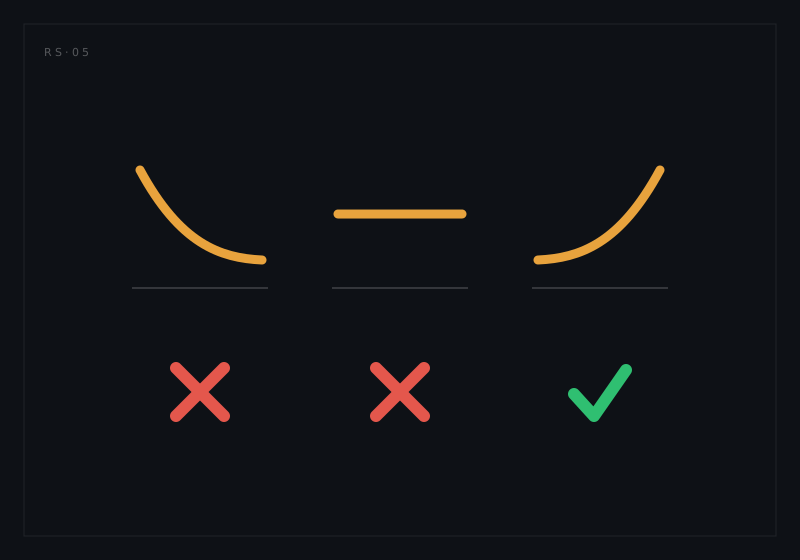
The shape parameter used above belongs to a Weibull distribution, which describes the time to failure of items that are not repaired: a bearing, a lamp, a capacitor, or the first failure of anything at all. Below one, the hazard falls with age, which is the early-failure signature. At one it is constant. Above one it rises, which is wear-out.
A repairable system that fails and is fixed repeatedly is a different mathematical object and has its own model: the power law non-homogeneous Poisson process, familiar to most engineers as Crow-AMSAA, with a failure intensity of the form λβt^(β-1). Its beta carries an analogous meaning, above one for a system whose failures are growing more frequent and below one for a system that is improving, which is why the same model underpins reliability growth work.
The trap is that both parameters are called beta, and fitting a Weibull to the successive failure times of one repairable system is among the most common errors in the discipline. On a data set where early years differ sharply from later ones, the two approaches can point in opposite directions.
The vocabulary splits the same way. MTBF belongs to repaired items and MTTF to items that are not repaired. IEC 61703:2016 sets out the mathematical expressions for these measures as defined in IEC 60050-192:2015, and the distinction is not pedantry: it decides which model you are entitled to fit in the first place.
Ask for the shape, not the mean
Once the shape is visible, the right action for each system is obvious, and it is different in each case.
The early-failure system needs screening: burn-in, incoming inspection, supplier process control. Spares do not fix it, they only move the cost around.
The steady system needs a spares pipeline, repair capacity and an honest availability model. What it does not need is scheduled replacement. Replacing a constant-hazard item on a calendar buys nothing, because a unit that has survived this far is in exactly the condition of a new one. That conclusion follows directly from the shape, and it is one of the foundations of reliability-centred maintenance.
The wear-out system is the single case where preventive replacement genuinely pays. It needs a life limit set from the distribution and enforced before the cliff, not after the first fleet-wide surprise.
So the thing to ask for, in a specification or from a supplier, is not a bare MTBF. Ask for reliability at a stated mission time, R(t) for a t that matters to the operation. Ask for a B10 or L10 life. Ask for the hazard trend and the data behind it. Ask which operating profile the numbers belong to. All four are answerable, and a supplier who can offer only a single number has told you something useful about how hard they looked.
How RAMSynapse approaches this
Most of the damage described here happens when a distribution is flattened into a single number early, and every analysis downstream inherits the flattened version. We built RAMSynapse so the shape survives the journey.
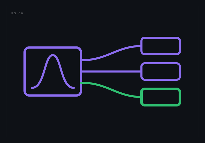
Weibull fits computed from FRACAS evidence stay attached to the item as distributions rather than being reduced to a mean on the way out. The maintenance and sparing analyses read that shape, so a life limit is proposed where the hazard rises and not where it does not. When new field data changes a fit, the analyses that consumed it recompute, and the trend itself is visible rather than buried in an average that has quietly stopped describing the fleet.
MTBF is not a bad metric. It is one summary statistic drawn from a distribution, and the distribution is where the engineering lives. Three systems can share the number and share nothing else, so the useful question was never what the MTBF is. It is which of the three you bought.
Want to see what your failure data says about the shape, and not just the mean? Request a walkthrough.