RAMSynapse
Log inSign up

RAMS Core

PublishedMIL-HDBK-217F Notice 2 · NSWC-11

Reliability Prediction

Parts-stress and parts-count failure-rate prediction — MIL-HDBK-217F Notice 2, NSWC-11 mechanical and related models.

Every reliability programme eventually has to answer one blunt question: how often will this design fail? The equipment does not exist yet, there is no fleet history, and yet the contract carries an MTBF number, the FMECA needs failure rates for its criticality arithmetic, the fault trees need basic-event probabilities, and the spares model needs demand rates. Reliability prediction is the analysis that produces those numbers before the hardware can produce them itself.

The method is old, standardised, and argued about — all three at once. At its core it is bookkeeping with physics sprinkled in: every part in the bill of materials is assigned a failure rate from a published model, the rate is adjusted for how hard the part is being worked and where it will serve, and the adjusted rates are summed up the product structure. The output — a system failure rate λ and its reciprocal MTBF — becomes the single most-consumed quantity in the entire RAMS workflow.

What a prediction is for is just as important as how it is computed. A handbook prediction is a consistent, comparable estimate of a mature design's inherent reliability — not a forecast of what the maintenance log will say. Programmes that understand this use predictions to compare architectures, expose the dominant contributors, and test compliance against allocated targets. Programmes that don't understand it end up defending a number that the field was never going to honour.

What it is and why it exists

Reliability prediction estimates the failure rate of equipment from the failure rates of its constituent parts, using standardised empirical models. The models were built by regression on large bodies of test and field data: for each part class — microcircuits, transistors, capacitors, connectors, relays — the data was fitted to a base failure rate plus a set of adjustment factors (the famous π factors) that capture how temperature, electrical stress, quality level, and application environment move the rate up or down.

The dominant reference is MIL-HDBK-217, "Reliability Prediction of Electronic Equipment", first published by the US military in the early 1960s and revised repeatedly as electronics evolved. The final revision is MIL-HDBK-217F (December 1991), amended by Notice 1 (July 1992, typographical corrections) and Notice 2 (28 February 1995), which revised the resistor, capacitor, connector, and interconnection models — including a surface-mount solder-joint model. Nothing has been issued since. An attempt to produce a revision G was launched in 2008 and abandoned; the handbook has been frozen for three decades while the components it models kept evolving. It also carries its own health warning on the cover: it is guidance, not a requirement, and its foreword says exactly that.

The handbook's own statement of purpose is worth internalising, because it defines the method's honest scope: to establish consistent and uniform methods for estimating the inherent reliability of mature designs, and to provide a common basis for comparing competing designs. Consistency and comparability — not clairvoyance.

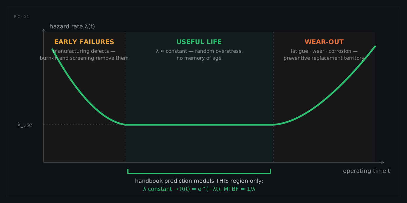
The bathtub curve. Handbook prediction models only the flat middle: a constant hazard rate λ, which makes reliability exponential in time. Early failures are a screening problem and wear-out is a maintenance problem — neither appears in a prediction.

The scope limitation that matters most is visible in the bathtub curve above. Handbook models assume a constant failure rate: the equipment is past its infant mortality (screened out by burn-in and manufacturing quality) and not yet into wear-out (managed by preventive replacement). Within that useful-life region the exponential distribution applies, the arithmetic becomes beautifully simple — rates add, MTBF is a reciprocal — and the model is blind, by construction, to anything that ages.

Electronic parts are only half the story. For mechanical equipment — springs, bearings, seals, gaskets, valves, actuators, pumps — the reference is the NSWC handbook of reliability prediction procedures for mechanical equipment (latest edition NSWC-11, May 2011, from the Naval Surface Warfare Center's Carderock Division). It works differently: instead of tabulated base rates, it computes failure rates from design and duty parameters — spring stress ratios, bearing loads, seal materials — through engineering equations. A programme with an electromechanical product typically runs both model families side by side, plus field-data compendia such as the NPRD/EPRD databooks for parts neither handbook models.

Where it sits in the programme

Prediction starts earlier than almost any other quantitative RAMS analysis and never really stops. At proposal stage, a parts count prediction produced from a preliminary parts list supports the bid's MTBF claim. Through detailed design, part stress predictions replace it, refreshed at every design revision as the BOM firms up and thermal and electrical analyses mature. After fielding, the prediction's job is to be progressively retired — replaced by observed rates from failure reporting and by life-data analysis, which are better evidence than any handbook.

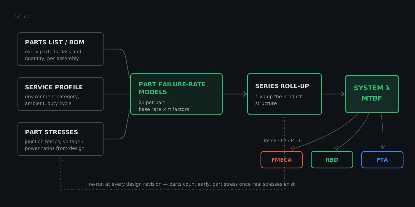
The prediction pipeline. Three input streams — the parts list, the service profile, and per-part stress data — feed part-level failure-rate models; a series roll-up produces the system λ and MTBF that the FMECA, RBD, and fault trees consume. The loop at the bottom is the method's real life: it re-runs at every design revision.

The analysis consumes three streams of input. The parts list comes from the design's bill of materials, with each part classified into a handbook category. The service profile declares where and how the equipment serves — environment category, ambient temperature, duty cycle, mission phases. The stress data comes from sibling engineering analyses: junction and hot-spot temperatures from thermal analysis, voltage and power stress ratios from the electrical design — the same ratios the derating analysis checks against its limits, which is why prediction and derating are natural companions: derating polices the stresses, prediction prices them.

Downstream, the prediction's outputs are the reliability programme's working currency:

  • FMECA — the criticality calculation of MIL-STD-1629A multiplies part failure rate, failure-mode ratio, and conditional probability (Cm = β·α·λp·t). The λp comes straight from the prediction.
  • RBD — reliability block diagrams take block failure rates from the prediction roll-up. The handbook itself is explicit that anything beyond a pure series structure — redundancy, duty cycles, mission profiles — is the modelling standard's territory, not the prediction's.
  • FTA — quantitative fault trees need basic-event rates; handbook predictions are one of their standard pedigrees.
  • Allocation — the prediction is the compliance test for allocated reliability budgets: allocation says what each block must achieve, prediction estimates what it will.
  • Logistics — spares provisioning, maintenance planning, and lifecycle cost all key off predicted failure rates until field data takes over.

This is exactly the wiring RAMSynapse draws on the live ring: the Prediction module publishes items and their FR/MTBF to the FMECA, and failure rates to the RBD and fault-tree modules, so a rate computed once is consumed everywhere without retyping.

Theoretical foundations

The quantities and their units

The primary quantity is the failure rate λ — the expected number of failures per unit of operating time. MIL-HDBK-217F expresses every rate in failures per 10⁶ hours; the telecom and European traditions (Telcordia, IEC, Siemens) work in FIT — failures per 10⁹ hours. Unit confusion between the two conventions is a classic audit finding, so keep the conversion at hand:

QuantityDefinitionConversion
λ (217F convention)failures per 10⁶ operating hours1 f/10⁶ h = 1,000 FIT
FIT (Telcordia / IEC convention)failures per 10⁹ operating hours1 FIT = 0.001 f/10⁶ h
MTBFmean operating time between failuresMTBF = 1/λ (constant-rate assumption)
R(t)probability of surviving to time tR(t) = e^(−λt)

Under the constant-rate assumption, MTBF is nothing more mysterious than the reciprocal of λ. A system predicting 20 f/10⁶ h has an MTBF of 50,000 hours — and, less intuitively, only a 37% chance of actually reaching 50,000 hours without failure, because e^(−1) ≈ 0.368. An MTBF is a mean, not a guarantee, and for exponential lifetimes the mean sits well past the median.

The constant-rate assumption and what it buys

The exponential distribution is the only lifetime distribution with a constant hazard rate — no memory, no ageing. Assuming it buys the method its entire algebra: failure rates of series elements add, so a system's rate is the sum of its parts' rates and the roll-up is a single pass of arithmetic up the product structure. It also defines the method's blind spots. A prediction cannot tell you when wear-out begins, cannot see batch-dependent infant mortality, and cannot represent a part whose risk grows with cycles rather than hours. Those questions belong to life-data analysis and physics-of-failure methods, not to the handbook.

Anatomy of a part-stress model. The handbook's typical form for discrete semiconductors: a base rate λb scaled by π factors, of which temperature, quality, and environment appear in almost every model. Microcircuits break the pattern with an additive die-plus-package structure.

The part failure-rate model

Each part category in the handbook has its own model, but the family resemblance is strong. The typical form — the handbook's own example for discrete semiconductors — is:

λp = λb · πT · πA · πR · πS · πC · πQ · πE

where λb is the base failure rate of the part class in its reference condition and each π factor scales it for one influence: πT temperature, πA application, πR power rating, πS electrical stress ratio, πC construction, πQ quality, πE environment. Quality and environment appear in nearly every model; the middle factors vary by part category — capacitor models bring capacitance and voltage-stress factors, resistor models bring power-stress factors, and so on.

Microcircuits are the notable exception, and the exception teaches the physics. Their model is additive at the core:

λp = (C1·πT + C2·πE) · πQ · πL

The die term (C1, scaled by temperature) and the package term (C2, scaled by environment) are separate because dies and packages fail differently: the die's failure mechanisms accelerate with junction temperature, while the package and its interconnects suffer from the vibration, humidity, and thermal cycling that the environment factor represents. Quality (πQ) and learning (πL — a penalty for devices in production less than two years) then scale the sum. In a benign environment the die term dominates; strap the same device to an airframe and the package term takes over.

The temperature factor is an Arrhenius exponential in junction temperature — πT = 1 at the 25 °C reference and roughly doubling every 25 °C in this activation-energy class. Temperature is the strongest lever a designer owns over predicted rate.

Temperature — the Arrhenius factor

The temperature factor deserves its own treatment because it is the strongest lever in the model and the one the design team can actually pull. Its kernel is the Arrhenius relationship — the same form chemistry uses for reaction-rate acceleration:

πT = exp[ −(Ea/k) · (1/TJ − 1/298) ]

with Ea the effective activation energy of the technology (electron-volts), k the Boltzmann constant (8.617×10⁻⁵ eV/K), and TJ the worst-case junction temperature in kelvin. At the 25 °C reference the factor is 1; above it, the rate climbs exponentially. Activation energies differ by technology — the handbook tabulates them per device family — so the steepness of the curve differs too; the microcircuit sections additionally carry a leading coefficient of 0.1 in their published πT expression, one of several reasons to read each part section rather than assume one formula fits all.

The junction temperature itself is an input, not a guess. The handbook's procedure is explicit: get case temperatures from a thermal analysis of the equipment, then compute

TJ = TC + θJC · P

— case temperature plus thermal resistance times dissipated power. If no thermal analysis exists yet, the handbook supplies default case temperatures per environment (45 °C for sheltered naval service, for example) — defaults that are exactly what the part-stress pass exists to replace with real numbers.

Quality and environment

The quality factor πQ encodes procurement class and screening depth, and its range surprises people seeing the method for the first time. For microcircuits the handbook's levels run from full space-grade screening to unscreened commercial parts:

Microcircuit quality levelπQDiscrete semiconductor levelπQ
Class S (space-grade screening)0.25JANTXV0.70
Class B (full military screening)1.0JANTX1.0
Class B-1 (MIL-STD-883 compliant)2.0JAN2.4
Commercial / unknown screening10Lower quality5.5
Plastic encapsulated8.0

A factor of 40 separates a space-grade microcircuit from an unscreened commercial one — in the model's eyes, procurement policy moves predicted reliability more than most design decisions. (The commercial-parts penalty is also the loudest single point of contention between the frozen 1995 models and modern component quality; more on that under pitfalls.)

The environment factor πE places the equipment in one of fourteen service categories, from benign ground installations to gun-launched projectiles:

CodeEnvironmentTypical service
GBGround, benignair-conditioned equipment rooms, laboratories
GFGround, fixedsheltered but unconditioned installations
GMGround, mobilewheeled and tracked vehicles
NSNaval, shelteredbelow-deck, sheltered shipboard bays
NUNaval, unshelteredexposed topside shipboard equipment
AICAirborne, inhabited, cargotransport-aircraft crew compartments
AIFAirborne, inhabited, fighterfighter cockpit environments
AUCAirborne, uninhabited, cargotransport equipment bays
AUFAirborne, uninhabited, fighterfighter equipment bays
ARWAirborne, rotary winghelicopters, internal and external
SFSpace, flightorbital operation
MFMissile, flightfree-flight missile phase
MLMissile, launchlaunch, boost, and re-entry loads
CLCannon, launchgun-launched guided projectiles

The spread is enormous: for microcircuits the environment factor runs from 0.5 in benign ground service to 220 for cannon launch. Choosing the environment category is therefore one of the highest-leverage decisions in the whole analysis — and one of the easiest to get subtly wrong when equipment spends its life in more than one of them.

The method, step by step

Two methods, one trajectory. Parts count needs only classes, quantities, quality, and environment — defaults stand in for stresses. Part stress replaces the defaults with the design's real temperatures and ratios. Every programme walks from the first to the second.

The handbook offers two procedures, and a real programme uses both — in sequence, not in competition. Parts count is the early method: it needs only the generic part types, their quantities, quality levels, and the equipment environment, with handbook defaults standing in for every stress. Part stress is the mature method: it needs the real electrical and thermal stress on every part, and it is only possible once the design can supply them. Parts count usually errs conservative — its defaults are deliberately unflattering — so the walk from one to the other typically earns back margin.

1. Choose the model set deliberately

The first decision is which models the programme will run, and it should be a contract-conscious one — mixed pedigrees in one roll-up need to be declared, because different handbooks embed different assumptions and units:

Model setDomain and character
MIL-HDBK-217F Notice 2Military electronics; parts count + part stress; frozen 1995; contractually entrenched
Telcordia SR-332 (Issue 4, 2016)Telecom/commercial lineage (ex-Bellcore); FIT units; first-year multipliers; can blend lab and field data into the estimate
IEC 61709:2017 / SN 29500European industrial practice: Siemens' reference-condition rates converted to application conditions via IEC stress models
FIDES (2022 edition)French aerospace/defence consortium guide; physics-of-failure-informed; mission-profile-driven, with an explicit process-quality audit factor
217Plus:2015Successor lineage to 217 (via RAC/RIAC); adds operating-profile and process-grade factors; supports Bayesian merge with own data
NSWC-11Mechanical equipment; engineering equations from design and duty parameters, not tabulated part rates
NPRD / EPRD databooksField-observed rates for parts no parametric model covers; gap-filler, not a model

Two companions are worth knowing whichever set you choose: ANSI/VITA 51.1 standardises input assumptions for 217F Notice 2 so that two analysts produce the same number from the same design, and IEEE 1413 is a framework for documenting a prediction — inputs, assumptions, data pedigree, uncertainties — so the number arrives with its provenance attached.

2. Frame the item and its mission

Define what is being predicted and where it serves. Select the environment category — and if the equipment sees more than one environment in use, segment the analysis: predict each mission phase in its own environment and time-weight the results by phase duration. The same goes for duty cycle: hours in the model are operating hours, and equipment that is energised 30% of the calendar needs that reflected, either in the profile or in how the result is quoted. This framing step is cheap, and errors in it are the expensive kind — they multiply everything downstream.

3. Build the part inventory

Pull the BOM into a part-class inventory: every line classified into a handbook category, with quantity, quality level, and — where the class needs it — complexity data such as gate counts, memory size, or package pin counts. This is data plumbing, and it is where a connected system model pays for itself: predictions built on hand-retyped BOM extracts inherit every transcription error and go stale at the first engineering change.

4. Run the parts count pass

The parts count equation is a single sum:

λ_EQUIP = Σ Nᵢ · (λg · πQ)ᵢ

— quantity times generic rate times quality factor, summed over the part categories (microcircuits pick up the learning factor πL as well; equipment spanning several environments computes per-environment and sums). The output is an early, defensible, usually conservative estimate — exactly what a proposal or an architecture trade needs.

5. Collect the real stresses

As the design matures, gather what the part-stress models need: worst-case junction temperatures from the thermal analysis (TJ = TC + θJC·P per part), applied-to-rated voltage and power ratios from the electrical design, application details per part category. Two handbook ground rules matter here: base rates may be interpolated between tabulated electrical stress values, but extrapolating beyond the tables — stress ratios above 1.0, temperatures beyond the tabulated range — is invalid. A part outside the tables is not a modelling problem; it is a derating finding that belongs in front of the design team.

6. Run the part stress pass and roll up

Compute λp per part from its category model, then roll up: sum the part rates per board, add the board-level contributions the handbook models separately — the printed wiring assembly, its solder connections, the connectors — and sum boards into units and units into the system. (Interconnecting wire between connectors is carried at zero rate; the connectors themselves are not.) The result is the system λ and MTBF, now traceable part by part.

7. Document, compare, iterate

Record the assumptions — environment, temperatures, quality claims, data sources per part — with the result. Compare against the allocation. Then expect to do it all again: every design revision, every BOM change, every updated thermal analysis moves the number. A prediction is not a milestone deliverable that gets archived; it is a living estimate that tracks the design until field data retires it.

Worked example

Consider a navigation data processor for a coastal patrol craft — an electronics box in a sealed below-deck bay, naval sheltered (NS) environment, three boards: a processor board, a power supply board, and an I/O board. The programme's allocation gives the box an MTBF budget of 40,000 hours. Every rate below is an illustrative teaching value chosen to walk the arithmetic; in a real study each λg and π comes out of the handbook tables for the exact part and conditions.

The parts count pass, board by board (rates in failures per 10⁶ h):

BoardPart classNλgπQN·λg·πQ
A · ProcessorMicroprocessor, 32-bit CMOS10.5601.00.560
A · ProcessorSRAM, 4 Mbit20.4101.00.820
A · ProcessorFlash, 64 Mbit10.4801.00.480
A · ProcessorCrystal oscillator11.2502.12.625
A · ProcessorCeramic capacitors460.00413.00.566
A · ProcessorFilm resistors380.00143.00.160
B · PowerDC-DC converter hybrid13.2001.03.200
B · PowerPower MOSFETs40.1802.41.728
B · PowerSchottky diodes60.1202.41.728
B · PowerTantalum capacitors120.06303.02.268
B · PowerPower inductors40.03003.00.360
C · I/ORS-422 transceivers60.2401.01.440
C · I/OOptocouplers80.3101.02.480
C · I/OCircular connectors, 55-pin20.5201.01.040
C · I/OBoard-edge connectors30.3101.00.930
C · I/OLED indicators50.03501.00.175

Summing per board and up to the system:

Levelλ (f/10⁶ h)Share
Board A — Processor5.21125.3%
Board B — Power9.28445.2%
Board C — I/O6.06529.5%
System20.560MTBF ≈ 48,600 h
The worked example rolled up. Three boards sum to a system rate of 20.56 failures per 10⁶ hours — an MTBF of roughly 48,600 hours against a 40,000-hour allocation. The power board owns 45% of the total, which is where the design conversation starts.

The headline: λ = 20.56 f/10⁶ h, MTBF ≈ 48,600 h — the box meets its 40,000-hour allocation with about 21% margin. But the roll-up's real product is the Pareto underneath it. The power board carries 45% of the system's failure rate; within it, the switching devices and the DC-DC hybrid dominate, and the twelve tantalum capacitors contribute more than the entire processor complex. The single worst part in the box is the crystal oscillator, whose commercial-grade quality factor more than doubled its contribution. Three actionable findings from one afternoon of arithmetic — before any hardware exists.

Refining one part with the part-stress model

Now the thermal analysis arrives and reports the microprocessor's worst-case junction temperature: TJ = 88 °C. The microcircuit part-stress model is λp = (C1·πT + C2·πE)·πQ·πL. Walking it through with illustrative coefficients — C1 = 0.28 (die complexity), C2 = 0.055 (package), πE = 4.0 (NS, microcircuits), πQ = 1.0 (Class B), πL = 1.0 (mature production):

First the temperature factor, using the microcircuit form with its 0.1 coefficient and a 0.35 eV activation energy (digital MOS class):

  • 1/TJ − 1/298 = 1/361 − 1/298 = −5.856×10⁻⁴
  • −(Ea/k) × that = −(0.35 / 8.617×10⁻⁵) × (−5.856×10⁻⁴) = 2.379
  • πT = 0.1 × e^2.379 = 1.08

Then the model:

λp = (0.28 × 1.08 + 0.055 × 4.0) × 1.0 × 1.0 = 0.302 + 0.220 = 0.52 f/10⁶ h

Two things worth noticing. The part-stress result (0.52) sits close to the parts-count default (0.56) — this box's thermal design is about as good as the handbook's average assumption. And the package term (0.22) is a fixed cost the environment sets: even a perfectly cooled die keeps it.

The model earns its keep in sensitivity. Suppose a packaging change blocks the airflow and TJ climbs to 110 °C: the same arithmetic gives πT = 2.06 and λp = 0.80 — a 53% increase in the part's failure rate from 22 degrees of temperature. That is the Arrhenius lever in action, and it is exactly the kind of quantified argument that wins a thermal-design debate.

Reading the results

The first rule of reading a prediction comes from the handbook itself: never assume the predicted number represents the field reliability the user will measure. The models are point estimates regressed from historical data under specific conditions; a National Academies review of the method collects case studies where measured-to-predicted ratios ranged from roughly one-half to twelve, and worse in extremes. The number's power is relative, not absolute — and the handbook says so in as many words.

Read relatively, the prediction answers real questions with real authority:

QuestionWhere to look
Does the design meet its allocation?System λ vs the allocated budget, with margin quantified
Where is the reliability going?The Pareto of contributors — boards, then parts, then factors
Which design change is worth it?Delta between predictions of the current and proposed design
Is the thermal design adequate?πT sensitivity of the hot parts; TJ excursions priced in failures
Is the parts policy right?πQ leverage — what screening buys, what commercial grades cost
Where does redundancy pay?Blocks whose predicted rates break the availability model downstream

The comparison discipline is what makes these answers trustworthy: two predictions compared under the same models, environments, and assumptions cancel most of the handbook's absolute error. That is why the method survived its critics — an obsolete model can still rank two architectures correctly, and ranking is what most programme decisions actually need.

One number deserves special respect: the margin against allocation. A prediction that lands under its budget is not a curiosity — it is an early warning with time still on the clock. The response is ordered and familiar: attack the Pareto leaders (cooler, softer-driven, better-screened, or fewer parts), renegotiate the allocation across siblings if one block is structurally hard, or escalate to an architecture change while one is still affordable.

Common pitfalls

PitfallWhat it looks likeThe guard
Selling the number as a field forecast"The prediction says 48,600 h, so the fleet will see it"Quote predictions as comparative estimates; track field MTBF separately
Unit mix-upsFIT and f/10⁶ h blended in one roll-up — a factor of 1,000Declare units at the top; convert at the boundary, once
One environment for a multi-phase lifeA missile electronics box predicted entirely in GFSegment the mission; time-weight per-phase results
Extrapolating the modelsStress ratios above 1.0, temperatures past the tablesTreat out-of-table parts as derating findings, not inputs
Forgetting the unglamorous contributorsNo PCB, solder-joint, or connector terms in the roll-upFollow the handbook's roll-up procedure to the letter
Optimistic quality claimsCommercial parts carried at military πQ "because the vendor is good"Evidence for the claimed screening, or the honest factor
Ignoring duty cycle and dormancyCalendar hours fed into operating-hour modelsDefine operating time explicitly; profile on/off phases
Chasing the number, not the designAssumptions tuned until the target is metThe handbook's own warning: those who treat the prediction as a number to exceed will find a way — without improving anything
Frozen-handbook blindness1995 models applied to parts that did not exist in 1995Say so in the assumptions; consider newer model sets or field data for modern parts

Most of these are process failures, not mathematics failures, and the last two deserve a sentence each. The gaming problem is old enough that the handbook warns about it explicitly — a prediction whose assumptions were tuned to clear a threshold has spent its credibility for one review meeting. And the frozen-handbook problem is structural: MIL-HDBK-217F Notice 2 predates three decades of component evolution, which is precisely why the serious modern practice is to treat handbook predictions as one pedigree among several — blended with field data where it exists, cross-checked against newer model sets where it matters, and always documented with their assumptions attached.

How RAMSynapse approaches this

RAMSynapse's Reliability Prediction module implements both procedures — parts count and part stress per MIL-HDBK-217F Notice 2, plus NSWC-11 for mechanical equipment — on the platform's shared system model, so the part inventory the prediction runs on is the same structure the rest of the analyses see, not a spreadsheet extract of it.

The computed rates travel through the module registry rather than through retyping: the prediction publishes its items and failure rates to the FMECA (where they price the criticality numbers), and its FR/MTBF results to the RBD and fault-tree modules (where they quantify blocks and basic events). When a design revision moves a junction temperature and the prediction re-runs, the downstream analyses see the new rates with their provenance intact — which is exactly how a living estimate should behave.


Want to see this on a live system model? Request a walkthrough.