

Availability composes across a system the way reliability does, with one deep difference: repair is part of the state. A reliability structure only asks which items are working; an availability structure also asks who is fixing what, with which crew, detected how quickly. That extra dimension is what makes repairable-system modelling its own craft, and what decides whether the simple product rules apply or a state model must take over. This chapter covers the composition rules and their fine print, works a radar station end to end, and turns the result into the budgeting discipline that makes availability targets manageable.
The composition rules
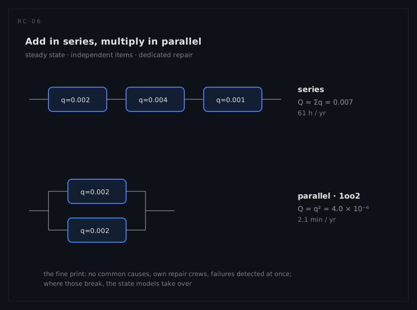
For steady-state availability with independent items, the structure rules mirror reliability's, and they are cleanest in unavailability terms, writing q = 1 − A:
- Series (all items needed): availabilities multiply,
Asys = ΠAᵢ; for small q this is the addition ruleQsys ≈ Σqᵢ. Downtime budgets in minutes per year therefore add straight down a series chain, which is what makes them allocatable. - Active parallel (any one suffices), each item with its own repair capability: unavailabilities multiply,
Qsys = Πqᵢ. This is redundancy's availability magic: two independent 99.8% channels make a 99.9996% pair, because the system is only down while both are down at once, and each failure's exposure window is only as long as its own repair. - k-out-of-n follows the same binomial logic as the reliability version, computed on the qᵢ.
The parallel rule's dependence on repair is worth pausing on, because it is the whole difference between availability redundancy and mission-reliability redundancy. The pair's unavailability is roughly the chance the second unit fails during the first one's repair: shorten the repair and the coincidence window shrinks with it. Redundancy and maintainability are therefore multiplicative allies: q² improves quadratically with everything that improves q, and a fast, well-provisioned repair loop is what keeps a redundant system living on the q² side of its arithmetic.
When the product rules break
Each product-rule assumption is a real-world failure mode:
| Assumption | How reality breaks it | What it does to the number |
|---|---|---|
| Independent failures | Common causes: shared power, cooling, software, environment (the CCF argument) | Floors Qparallel at the coupled fraction; q² becomes βq |
| Dedicated repair per item | One crew or one test stand shared across the site; repairs queue | Effective MDT grows with utilisation; the second failure waits |
| Immediate detection | Standby channel fails silently; found only at test | The pair runs as a single string for the latent interval; the λT/2 ledger from the foundations chapter applies |
| Instant, perfect switchover | Failover takes time, sometimes fails, sometimes disturbs the load | Every demanded switchover contributes its own downtime term |
When these couplings matter, the honest tool is a state model: enumerate the system's states (both up; one up, one in repair; both down; one up, one failed-undetected…), attach failure, repair, detection, and test transitions, and solve for state probabilities. That is Markov modelling, the availability world's workhorse for exactly the situations where "who is repairing what" changes the answer: shared crews, imperfect switching, latent failures, staged degradation. Its cost is state explosion on large systems, which is why practice layers the tools: product-rule arithmetic (RBD availability) across the broad system, Markov (or simulation, once logistics networks and spares stocks enter) zoomed onto the few redundant clusters where the couplings live. This chapter builds and solves those state equations below, on the same radar station.
The radar station, end to end
The overview's surveillance radar, worked as one table. A transmitter has MTBF 2,000 h and a 4-hour active repair; the station needs continuous coverage; all values are illustrative:
| Configuration | Per-channel downtime per failure | q per channel | Station unavailability | Downtime per year |
|---|---|---|---|---|
| Single channel, spare on site | 4 h | 0.0020 | 0.0020 | 17.5 h |
| Single channel, spare 2 days away | 48 h | 0.0234 | 0.0234 | 205 h |
| Dual channel, spares on site | 4 h | 0.0020 | q² ≈ 4.0 × 10⁻⁶ | 2.1 min |
| Dual channel, spares 2 days away | 48 h | 0.0234 | q² ≈ 5.5 × 10⁻⁴ | 4.8 h |
Four lessons, one table. Logistics dominates the single string: moving the spare off-site multiplied downtime twelvefold with identical hardware. Redundancy is spectacular but honest: the on-site duplex earns minutes per year, a factor of 500 below the on-site single string. Logistics follows the redundancy: the off-site duplex is 138 times worse than the on-site one, so moving the spares does to the pair exactly what it did to the single string. And the last row is still optimistic: it assumes both channels never share a power feed, a cooling fault, a software load, or a lightning strike, and that the standby channel's health is genuinely known (the previous section's fine print). Real dual-channel stations spend their engineering exactly there: separation, diversity where affordable, and built-in test that keeps the second channel's silence honest. Both duplex rows also assume that each channel has a repair capability of its own rather than sharing the site's one crew, which is the assumption the next section prices.
State models
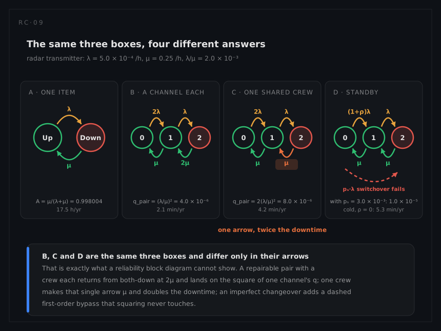
Those duplex rows were computed with the product rule, and the product rule was never told who repairs the second channel. A state model is what asks. Its machinery is small: enumerate the states the system can occupy, attach a transition rate to every arrow between them, and require that in the long run the probability flowing into each state equals the probability flowing out. One balance equation per state, plus the condition that the state probabilities sum to one, solves every model in this section by hand. The arithmetic is the easy part. The enumeration is the analysis, because it forces the repair channel, the detection interval and the switchover onto the page as explicit parameters rather than leaving them as assumptions nobody wrote down.
One item, two states. The foundations chapter asserted A = μ/(λ + μ); the two-state chain is where it comes from. A repairable item is either up or down, it leaves the up state at rate λ and the down state at rate μ = 1/MTTR, and because there is only one boundary between the two, the probability flow across it must balance:
λ × Pup = μ × Pdown
With Pup + Pdown = 1 that solves immediately:
A = Pup = μ / (λ + μ)
Q = Pdown = λ / (λ + μ)
Substituting λ = 1/MTBF and μ = 1/MTTR turns the rate form into the time form, which is the same statement in different units rather than a second formula to remember:
A = (1/MTTR) / (1/MTBF + 1/MTTR) = MTBF / (MTBF + MTTR)
For the station's transmitter, λ = 5.0 × 10⁻⁴ per hour and μ = 0.25 per hour:
A = 0.25 / (0.25 + 0.0005) = 0.998004 = 2,000 / 2,004
q = 1 − A = 4 / 2,004 = 1.996 × 10⁻³
1.996 × 10⁻³ × 8,766 = 17.5 hours a year
the first row of the table above, now derived rather than quoted. Two properties of the balance equation carry into everything that follows. Only the ratio λ/μ survives the reduction, which is the algebraic reason the trade space exists at all: halving MTTR and doubling MTBF are the same move on the same number. And the steady-state result needs only that a mean up time and a mean down time exist, so it holds whatever shape the two distributions have; the exponential assumption buys the transient A(t) and the multi-state chains below, not the limit. MIL-HDBK-338B carries this derivation with its shared-crew caveat, and IEC 61703 gives the state-transition forms of the same quantities.
Two units, and the one arrow that changes the answer. Take two identical repairable units in active parallel and index the states by how many have failed: 0, 1, 2. The failure arrows are identical in both repair regimes, because failures do not queue. The repair arrows are not:
| Transition | What happens | Dedicated repair, a channel per unit | One shared repair channel |
|---|---|---|---|
| 0 → 1 | either unit fails | 2λ | 2λ |
| 1 → 0 | that repair completes | μ | μ |
| 1 → 2 | the survivor fails during the repair | λ | λ |
| 2 → 1 | the first of two repairs completes | 2μ | μ |
Balancing state 1 gives P₁ = 2(λ/μ) × P₀ in both regimes. Balancing state 2 does not:
dedicated: P₂ = (λ / 2μ) × P₁ = (λ/μ)² × P₀
shared: P₂ = (λ/μ) × P₁ = 2(λ/μ)² × P₀
One arrow, one factor of two, and the whole difference between two support contracts that look the same on a block diagram. Both forms of P₂ are the same quantity the previous section described in words: the coincidence term, the probability that the second unit fails inside the first one's repair window.
The dedicated case is the product rule, and it is not an approximation of anything. Two items each holding its own repair capability are two independent alternating processes, so the probability that both are down is the product of the individual unavailabilities exactly, with each item's own q = MTTR / (MTBF + MTTR). Where every item has its own channel, Q = Πqᵢ is the answer and a state model adds nothing but effort.
The shared case is the one that gets left out of proposals. With one crew, one test stand or one dispatched field engineer serving the group, the second failure waits for the first repair to finish, and for a group of n units that is down only when all n are down the penalty against the product rule is a factor of n!, which is 2 on a pair and 6 on a triplex. The storage array's controller pair carries exactly that factor of two, for exactly that reason, because one engineer is dispatched under one service contract. A k-out-of-n group with a shared channel gets no such shortcut and needs its own chain.
Which regime applies is a procurement fact before it is an engineering one. Nothing in the hardware decides whether the site holds two crews or one, whether the second call-out is answered while the first repair is running, or whether the service agreement's response clock restarts for a concurrent fault; the support contract decides all three, and the availability model cannot honestly be written until someone has read it. A requirement quoted as q² is a requirement on the support arrangement as much as on the design.
The three standby questions a block diagram cannot ask. A structure diagram draws two boxes side by side whether the second one is running hot, barred and warm, or cold and unpowered; whether its health is known continuously or once a week; and whether the mechanism that brings it into service works when asked. A state model has to answer all three, and each answer is a different parameter.
- Dormancy. Let the waiting unit fail at ρλ while it waits, a fraction ρ of its running rate: ρ = 1 is a hot standby with identical exposure, ρ = 0 a true cold standby accruing nothing, and the warm cases sit between. Both units' failures lead to the same one-failed state, so the chain's first transition becomes (1 + ρ)λ and, with a single repair channel, the both-failed probability is
qpair = (1 + ρ)(λ/μ)² / (1 + (1 + ρ)(λ/μ) + (1 + ρ)(λ/μ)²), which is(1 + ρ)(λ/μ)²to leading order. Setting ρ = 1 recovers the shared-channel active pair at2(λ/μ)²; setting ρ = 0 recovers the cold-standby form(λ/μ)²/(1 + λ/μ + (λ/μ)²), and the two bracket every real standby. The energy train's barred lube oil pump sits at 1.1 × 10⁻⁵ against a cold-standby 9.0 × 10⁻⁶, which gives (1 + ρ) ≤ 1.22 and so ρ ≤ 0.22 once the changeover term that page also carries is set aside: a barred pump accruing at most about a fifth of its running rate while it waits. Note also what the endpoints do: a cold standby with one crew and an active pair with two both land on(λ/μ)², because the cold spare halves the exposure by exactly the factor the shared crew doubles it. - Switchover. The changeover is a demand on a mechanism, and it either works or it does not. Give it a failure probability
psper demand. The running unit's failure, arriving at rate λ, then takes the whole system down with probabilitypsand keeps it down for the restoration:qswitch ≈ ps × λ × MDT = ps × (λ/μ). That term is first order in λ/μ where the coincidence term is second order, which is exactly why it matters: redundancy's quadratic advantage does not apply to it, and it is invisible to any model built out of blocks. Take the nuclear diesel's measured start-on-demand failure probability of 3.0 × 10⁻³ aspsfor a transmitter held in cold standby, andqswitch = 3.0 × 10⁻³ × 2.0 × 10⁻³ = 6.0 × 10⁻⁶against a coincidence term of 4.0 × 10⁻⁶. The switch is 60% of the pair's unavailability, and improving the repair loop makes its share worse rather than better: at a two-hour restoration the pair sits at 4.0 × 10⁻⁶ with the switch carrying 75% of it. - Detection. Everything above assumes the standby's failure is known when it happens. Found instead by a periodic exercise, the waiting unit contributes not λ × MDT but the λT/2 sawtooth of the foundations chapter, and to leading order the pair's unavailability becomes a latent probability multiplied by a repair probability,
qpair ≈ (λT/2) × (λ × MDT). Confirm the second transmitter's health by a weekly built-in-test exercise rather than continuously (T = 168 h, illustrative like everything else here) and(5.0 × 10⁻⁴ × 168 / 2) × (5.0 × 10⁻⁴ × 4) = 0.042 × 0.0020 = 8.4 × 10⁻⁵. The ratio to the monitored pair is just the ratio of exposure windows,(T/2) / MDT = 84 / 4 = 21.
Six regimes for one pair of transmitters, at λ = 5.0 × 10⁻⁴ per hour, MDT = 4 h and λ/μ = 2.0 × 10⁻³ throughout:
| Regime for the second transmitter | Pair unavailability | Downtime per year |
|---|---|---|
| Active, a repair channel each | q² = 4.0 × 10⁻⁶ | 2.1 min |
| Active, one repair crew for the pair | 2(λ/μ)² = 8.0 × 10⁻⁶ | 4.2 min |
| Cold standby, one crew, perfect switch | (λ/μ)² = 4.0 × 10⁻⁶ | 2.1 min |
| Warm standby at ρ = 0.22, one crew | 1.22(λ/μ)² = 4.9 × 10⁻⁶ | 2.6 min |
| Cold standby, switch failing 3 demands in 1,000 | 4.0 × 10⁻⁶ + 6.0 × 10⁻⁶ = 1.0 × 10⁻⁵ | 5.3 min |
| Active, health confirmed weekly rather than continuously | (λT/2)(λ × MDT) = 8.4 × 10⁻⁵ | 44 min |
Every row is the same two transmitters, the same failure rate and the same four-hour repair; the regime alone moves the station's downtime by a factor of twenty-one, and a block diagram draws all six identically. The fifth row is worth a second look for where it lands: 1.0 × 10⁻⁵ is the five-nines line from the overview's ladder, and it got there from a switch that works 997 times in 1,000, not from anything that failed.
Every coincidence term above goes as the square of λ/μ, so restoration time enters squared there; the switchover and latent terms of the previous section are first order in MDT and only halve when it halves. Halving the transmitter's four-hour repair to two hours takes the shared-channel pair from 8.0 × 10⁻⁶ to 2.0 × 10⁻⁶, 4.2 minutes a year down to 1.0; doubling it to eight hours costs 16.7 minutes; and the off-site spare's 48-hour restoration takes the same pair to 1.1 × 10⁻³, 9.6 hours a year, 276 times the on-site duplex with dedicated crews. Failure rate is quadratic in precisely the same way, since only the ratio appears: doubling MTBF and halving MDT buy the identical factor of four, the foundations chapter's trade space squared. What separates them is the purchase order rather than the mathematics. MDT is bought from the support system in weeks, by moving a spare or adding a shift; λ is bought from the design, in a redesign cycle. On a repairable redundant pair, halving the restoration time is worth exactly what doubling MTBF is worth, and no model without repair transitions can show it, because it has nowhere to put MDT.
When the product rules are legitimate. The point of a state model is to be used sparingly, and the test for when it is needed is the order of the leading term:
- Series chains compose freely, in any repair regime. The answer is first order,
Qsys ≈ Σqᵢ, and repair coupling only bites while the chain is already down, a fraction of order q of the time. For two series items at q = 2.0 × 10⁻³ the sum is 4.0 × 10⁻³ and the coupling correction is of order q² = 4.0 × 10⁻⁶: one part in a thousand, far below the accuracy of any failure rate feeding it. - Redundant groups with a dedicated repair channel each compose exactly.
Q = Πqᵢis the answer, and a state model returns the same number after more work. - Redundant groups sharing a repair channel take the n! factor, provided the channel is the only coupling. Solve the cluster, collapse the result into an equivalent q, and hand that q back to the surrounding block diagram: that is what makes the state model a zoom lens rather than a competing model of the whole system (the methods chapter draws the same boundary).
- Imperfect switching, latent failures and staged degradation admit no correction factor at all. Their terms are first order in λ/μ where the coincidence term is second order, so they do not scale with the rest of the model and cannot be folded into a q that a structure diagram will then square. These are the clusters that must actually be enumerated.
- Common cause is not a repair problem, and no amount of repair modelling removes it; a chain can carry a direct both-failed transition at βλ, but the floor it puts under the answer comes from separation and diversity, not from the solver.
The β floor from the reliability systems chapter sits underneath every number in this section: solving a three-state chain to three significant figures while both channels share a power feed is precision spent in the wrong place.
Enumeration is also where the cost sits. Identical units can be lumped by how many have failed, which is why the pair above is three states rather than four and a triplex is four rather than eight, but the lumping dies the moment the units differ, or the moment a state has to remember which unit failed first, or which failures are announced and which are not. That is the state explosion, and it is the reason the honest practice is the layered one: product-rule arithmetic across the system, a solved chain on each cluster where the couplings live, and the cluster's answer carried back out as a single number.
Budgeting downtime
An availability requirement becomes manageable the moment it is converted into a downtime budget and allocated like any other budget: the station's 99.95% becomes 4.4 hours per year, split across the antenna group, transmitters, processing, power, and communications in minutes, each line owned by a designer who can trade failure rate against repair time against sparing inside it. Because small unavailabilities add in series, the ledger arithmetic is as simple as reliability allocation's, with one extra column: every line's q decomposes into an MTBF part, an MTTR part, and an MLDT part, so the budget simultaneously constrains the design and the support system.
Planned downtime deserves its own ledger line rather than an exclusion clause. The nuclear exemplar from the overview is the discipline at its most mature: a refuelling outage is a project with a critical path, planned years ahead, rehearsed, and compressed by parallelising every task that maintenance task analysis can take off the chain, because each saved hour is an hour of production bought at planning cost. The general rule scales down from there: scheduled work should be aggregated into windows, moved off the operational calendar where the mission allows, and designed for (the design chapter returns to hot-swap and online-maintenance architecture); a budget that only tracks unscheduled downtime quietly hands the schedulers an unlimited account.