

Availability's mathematics is the mathematics of an alternating process: a repairable item cycles between up and down states, and every availability measure is some ratio carved out of that cycle. The subtlety is never the arithmetic; it is the bookkeeping. Which clock counts as uptime, which delays count as downtime, and over what window the ratio is taken: those three decisions generate the whole family of availability measures, and confusing two family members is the field's most common error. This chapter builds the family precisely, dissects downtime into its owned parts, and covers the hidden form of unavailability that no uptime log ever shows.
Notation used in this topic
| Symbol | Reads as | Meaning |
|---|---|---|
| A(t) | point availability | probability the item is up at instant t |
| A | steady-state availability | the long-run limit, μ/(λ+μ) |
| Q, q | unavailability | 1 − A; the working currency, because small values add in series |
| Ai, Aa, Ao | inherent, achieved, operational | the three named availabilities, differing in what counts as downtime |
| Am | materiel availability | the fleet-wide form, including units in depot or reserve |
| λ, μ | lambda, mu | failure rate and repair rate |
| MTBF, MTBM | mean time between failures, and between all maintenance actions | |
| MTTR, MDT | mean active repair time, and mean downtime including all delays | |
| LDT, MLDT, ADT | logistics delay time and its mean, and administrative delay time | |
| T | proof-test interval | the period between exercises of a dormant function |
Every abbreviation used anywhere in RAMS Core is defined in the glossary.
The availability functions
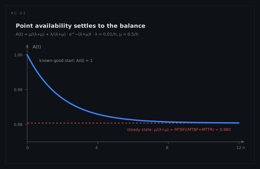
Let a single item alternate between working and being restored, with constant failure rate λ and constant repair rate μ (mean repair time 1/μ). Three time-flavours of availability follow:
- Point (instantaneous) availability A(t): the probability the item is up at instant t. For the constant-rate model it has a closed form,
A(t) = μ/(λ+μ) + λ/(λ+μ) · e^−(λ+μ)t, starting at 1 and settling exponentially to its limit. - Mean availability over an interval: the expected fraction of the interval spent up; what a monthly report actually computes.
- Steady-state availability A: the long-run limit,
A = μ/(λ+μ) = MTBF/(MTBF + MTTR), the single most-quoted formula in the discipline. Its structure carries the trade space: only the ratio of repair to failure time matters, so halving MTTR buys exactly what doubling MTBF buys.
The unavailability Q = 1 − A is often the better working currency, for the same reason failure rates beat reliabilities in series arithmetic: when q is small, contributions add. A system's downtime budget in minutes per year is just Q × 525,960, and budgets that add are budgets that can be allocated.
The three classic forms
The military handbooks (MIL-HDBK-338B, MIL-HDBK-470A) standardised three named availabilities, distinguished by what the denominator's downtime includes:
| Form | Formula | Counts as downtime | Who owns the number |
|---|---|---|---|
| Inherent Ai | MTBF / (MTBF + MTTR) | Active corrective repair only; ideal support, no delays, no preventive maintenance | The design (reliability + maintainability) |
| Achieved Aa | MTBM / (MTBM + M̄) | Corrective and preventive maintenance, still ideal support | Design + the maintenance policy |
| Operational Ao | uptime / (uptime + downtime), i.e. MTBM / (MTBM + MDT) | Everything: repairs, preventive work, logistics delay, administrative delay | The whole enterprise |
Reading the table downward is reading responsibility outward. Ai is the design's promise and the only form a factory demonstration can verify. Aa penalises designs that demand frequent or long preventive attention, which is why "maintenance-free" architectures score their gains here. Ao is the truth: the number the mission feels, the number defence support arrangements are written against, and the only one that notices whether the spare was on the shelf. (At programme level the formal sustainment key performance parameter is materiel availability, computed across the whole fleet including everything in depot; Ao is the operating unit's view of the same idea.) The three are not competing definitions but one system viewed with progressively fewer excuses, and a healthy programme quotes them together: a wide Ai-to-Ao gap is a support-system finding, not a design finding.
One bookkeeping rule prevents most availability disputes: publish the clock definitions with the number. Whether a degraded mode counts as up, whether a planned outage window is excluded, whether "awaiting parts" pauses the downtime clock: each choice can move the reported availability by more than the engineering did. The measure is only as honest as its ledger.
Downtime, dissected
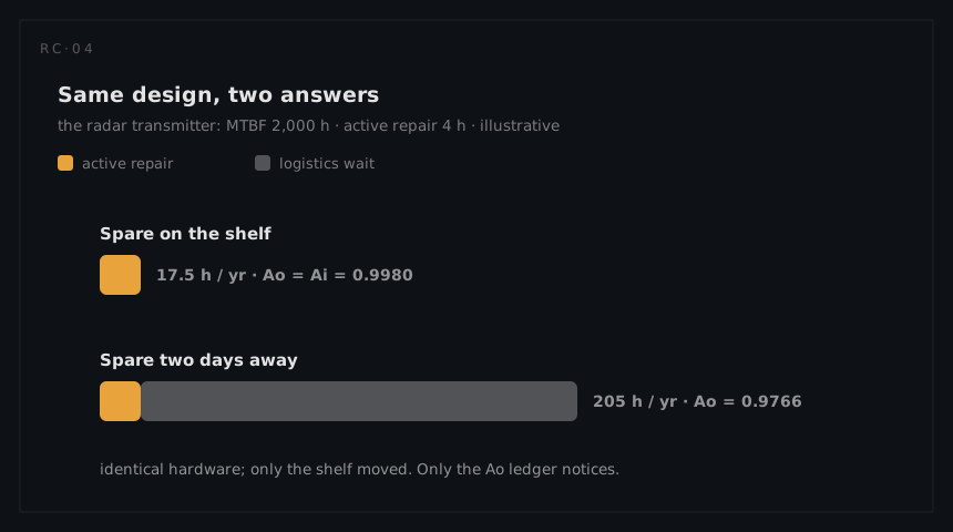
Operational availability's denominator, mean downtime (MDT), decomposes into parts owned by different budgets:
MDT = active repair time + logistics delay + administrative delay
- Active repair is maintainability's territory: diagnosis, access, interchange, verification, the part of downtime the design controls.
- Logistics delay time (LDT, with its mean MLDT) is the support system's: waiting for spares, for the right technician, for transport, for test equipment. In fielded systems it routinely dwarfs the wrench time, which is why the DoD's availability guidance breaks it out as its own named quantity.
- Administrative delay (ADT) is the organisation's: work-order processing, approvals, permits-to-work, priority queues, shift boundaries. It is the cheapest slice to fix and the most embarrassing to measure.
The decomposition is what makes the Ai-to-Ao gap actionable. A single worked pair carries the whole lesson (the same numbers return in the systems chapter): a transmitter with a 2,000-hour MTBF and 4-hour repair has Ai = 0.9980, about 17.5 hours of downtime per year. Put its only spare a two-day shipment away and each failure now costs 48 hours: Ao = 0.9766, over 200 hours per year, a twelvefold collapse with identical hardware. Buying a second spare shelf is, in that regime, worth more than any feasible component upgrade, and only the Ao ledger can reveal it.
Hidden unavailability: on-demand systems
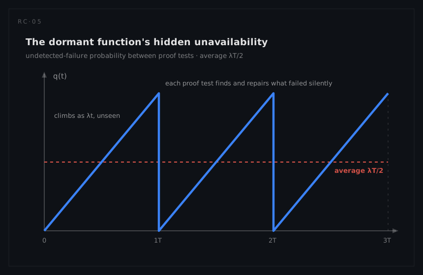
Everything above assumed failures announce themselves. A protective or standby function inverts the picture: it sits dormant, its failures are silent, and its availability question is will it work when demanded? The uptime ledger is useless here; a tripped-breaker function can be "up" on every dashboard and dead for six months.
The governing model is the periodically tested dormant unit. If undetected dangerous failures arrive at rate λ and a proof test every T hours finds and repairs them, the unavailability seen by a random demand climbs from zero after each test to λT just before the next, averaging
Qavg ≈ λT / 2 (for λT ≪ 1)
This is the quantity functional-safety practice calls the average probability of failure on demand (PFD) for a low-demand safety function, the currency of the IEC 61508 tradition and the nuclear protective-system world from the overview. Three engineering consequences follow. The test interval is an availability parameter, as powerful as the failure rate and far cheaper to change: halving T halves the hidden unavailability. Testing has its own costs: each proof test takes the function out of service briefly, can itself induce failures, and at some frequency the test downtime and test-caused failures overwhelm the latent-risk gain; there is an optimum interval, not a "more is better" rule. And detection converts the problem: any failure the built-in monitoring reveals immediately moves from the λT/2 regime to the ordinary announced-failure regime, which is why testability coverage appears inside availability arithmetic, and why a redundant pair with an undetected failed channel is quietly running as a single string (the redundancy exposure argument).
Measuring availability in service
Operational availability is ultimately an observed quantity, and observation has failure modes of its own. The recurring ones: window games (annual averages burying a catastrophic month; measuring across the fleet to hide the one chronically-down unit, which is why fleet-level materiel availability and unit-level Ao are tracked as separate indicators); ledger games (reclassifying downtime as "excluded" categories: awaiting parts, awaiting access, customer-caused); partial-state ambiguity (a system at half capability counted as fully up, common wherever capacity rather than binary function is the product, which is why process industries track production-weighted availability and the power sector uses energy-based availability factors rather than clock-based ones); and numerator optimism (counting standby time as up without any demand or test having proven it, the hidden-unavailability trap again).
The defences are procedural, not mathematical: definitions published before the first report, downtime categorised at the event by cause (design, maintenance, logistics, administration) so the FRACAS loop can route each hour to its owner, and periodic reconciliation of the observed Ao against the model that predicted it. The comparison of predicted against observed availability is the sharpest audit a support system ever gets: the failure-rate part of the error indicts the prediction, the repair-time part indicts the maintainability analysis, and the rest is the logistics ledger explaining itself.