

Maintainability's quantitative core mirrors reliability's with the clock reversed: instead of asking how long a working item survives, it asks how long a failed item stays failed. Repair completion time is the random variable, a distribution describes it, and everything a programme quotes (MTTR, percentile times, downtime, man-hours) is a summary of that distribution. This chapter builds the machinery: the maintainability function, the point measures and their traps, the anatomy of a corrective action, the distributions that fit real repair data, the preventive branch and the combined maintenance ledger that availability draws on, and how the numbers are estimated and demonstrated.
Notation used in this topic
| Symbol | Reads as | Meaning |
|---|---|---|
| M(t) | maintainability function | probability the maintenance action is complete by t |
| μ | mu | repair rate, the mirror of λ; mean repair time is 1/μ |
| MTTR, M_ct | mean active corrective time at a stated level of repair | |
Mmax | maximum corrective time | a percentile of the repair-time distribution, usually the 90th or 95th |
| M_pt | mean time per preventive maintenance action | |
| M̄ | mean maintenance time | corrective and preventive combined, weighted by their rates |
| MTBM | mean time between maintenance actions of either kind | |
| MDT | mean downtime | active repair plus logistics delay plus administrative delay |
| MLDT | mean logistics delay time | waiting for spares, people, transport or test equipment |
| MMH/OH | maintenance man-hours per operating hour | the labour ledger, distinct from elapsed time |
| LRU, SRU | line- and shop-replaceable unit | what is exchanged at the line, and inside it at the shop |
tmed, σ | median, sigma | the lognormal repair-time parameters |
Every abbreviation used anywhere in RAMS Core is defined in the glossary.
The maintainability function
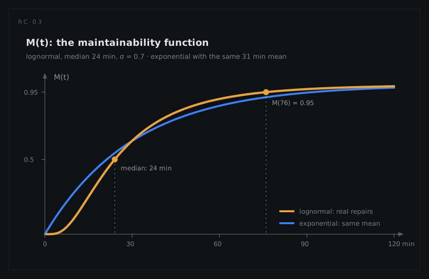
Let Tm be the time to complete a maintenance action, measured from its start under stated conditions. The maintainability function M(t) = P(Tm ≤ t) is the probability that the action is finished by elapsed time t. It is the mirror image of the reliability function: R(t) starts at 1 and falls as failures accumulate; M(t) starts at 0 and rises as repairs complete. A maintainability requirement is a point pinned onto this curve: "90% of corrective actions complete within 60 minutes" is M(60 min) ≥ 0.90, no more and no less.
The analytic workhorse is the constant-repair-rate model. If completions arrive with constant rate μ among still-open repairs, then
M(t) = 1 − e^(−μt), with mean repair time 1/μ
exactly parallel to the exponential life model, and convenient for the same reason: it makes the availability mathematics linear and gives closed forms for repairable-system models. It carries the same warning label, too. Real corrective actions are not memoryless: a repair that has run three hours is usually a difficult repair, not a fresh one, so the true completion rate is not constant. The exponential repair model is an engineering convenience to be used where its errors do not matter (long-run availability arithmetic) and avoided where they do (percentile commitments, staffing decisions).
Point measures and their traps
| Measure | What it is | The trap |
|---|---|---|
| MTTR (or M_ct) | Mean corrective time: total active corrective time divided by the number of repairs, at a stated level of repair | Active time only, at one echelon; it is not the downtime the operator feels |
| M_pt | Mean preventive maintenance time per action | Often quoted per action while the burden driver is frequency × duration |
| M̄ | Combined mean maintenance time: corrective and preventive averaged by their rates | Falls when short frequent tasks are added, which is the opposite of an improvement |
| MTBM | Mean time between maintenance actions of either kind | Always shorter than MTBF; putting MTBF in its place overstates the up-cycle |
Mmax | Percentile corrective time, classically the 90th or 95th | The commitment that actually protects operations; a mean cannot |
| MDT | Mean downtime: active repair plus logistics delay plus administrative delay | The number availability actually feels; blaming MTTR for an MDT problem fixes the wrong thing |
| MLDT | Mean logistics delay time: waiting for spares, people, transport | A support-system property, not a design property; separate the ledgers |
| MMH/OH | Maintenance man-hours per operating hour | Labour, not elapsed time: three technicians for one hour is one hour of MTTR and three of MMH |
Two of these traps sink real programmes often enough to name explicitly. First, the mean-versus-percentile trap: repair-time distributions are strongly right-skewed, so the mean is dragged upward by a minority of long repairs and can sit far above the median. A fleet can meet a 40-minute MTTR while a repair in ten blows a two-hour maintenance window, which is why demanding requirements are written on Mmax percentiles, with MTTR as a companion. Second, the MTTR-versus-MDT trap: MTTR is a design property measured wrench-in-hand; downtime adds everything the support system wraps around it. Both matter, but they are owned by different people and fixed by different budgets. A contract that specifies only MTTR has quietly declined to buy short downtime.
Units carry the same discipline as reliability's: repair times in hours or minutes at a stated level of repair, man-hours as a separate ledger, and every number tagged with the maintenance conditions (skill level, tools, documentation state) it was measured under.
Anatomy of a corrective action
The corrective clock decomposes into task elements, and the decomposition is where design meets the stopwatch. The classic chain (the military handbooks enumerate localization, isolation, disassembly, interchange, reassembly, alignment, and checkout; preparation is the practical step in front of them):
| Element | The question it times | The design lever that compresses it |
|---|---|---|
| Preparation | Tools, safety isolation, documentation in hand | Standard tools, captive hardware, clear procedures |
| Fault localization | Which subsystem is misbehaving? | Monitoring, alarms, operator indications |
| Fault isolation | Which replaceable unit is at fault? | Built-in test resolution: the testability coverage numbers |
| Disassembly (access) | Can the unit be reached? | Layout, access panels, nothing-on-top-of-anything design |
| Interchange | Remove and replace the unit | Modularity, connectors over solder, guides and keying |
| Reassembly | Put the system back together | Fewness of fasteners, impossible-to-invert fits |
| Alignment and calibration | Does the new unit need tuning? | Self-calibration, stored settings, no-adjustment design |
| Checkout | Is the system verifiably healthy again? | Built-in verification, unambiguous pass indications |
The split matters because the elements respond to different investments, and because their weights have shifted historically: in electronics-dense systems the diagnosis pair (localization plus isolation) commonly dominates the total, which is why testability coverage is the first number to check when a predicted MTTR looks unreachable. The elemental times are also the raw material of prediction: maintainability prediction methods in the MIL-HDBK-472 lineage estimate a design's repair times by scoring or tabulating exactly these elements against the design's features, long before hardware exists to time.
Repair-time distributions
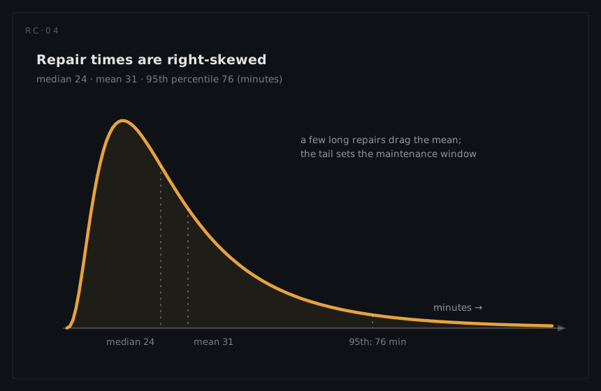
Repair-time data across industries shows a stubbornly consistent shape: most actions cluster around a typical value, and a long right tail of difficult cases (misdiagnosis, seized fasteners, missing spares, second faults found) stretches far beyond it. The lognormal distribution is the classic model for exactly this behaviour, and has been the default for corrective repair times since the discipline's military-handbook era. Its parameters read naturally: the median tmed is the "typical repair", and the shape σ measures the spread of the multiplicative factors that make real repairs run long or short. Key working relations:
mean = tmed × e^(σ²/2): the mean exceeds the median, always, by the tail's pulltp = tmed × e^(zp·σ): the percentile, withzpthe standard normal quantile
A worked instance shows the arithmetic a requirement writer needs. Take a repair population with median 24 minutes and σ = 0.7. The mean is 24 × e^0.245 = 30.7 minutes: already 28% above the median. The 95th percentile is 24 × e^(1.645 × 0.7) = 76 minutes: more than three times the median, and that, not 24 or 31, is the number a maintenance window must absorb. The same design would honestly report MTTR ≈ 31 min and Mmax(95%) ≈ 76 min, and both belong in the specification.
| Distribution | Where it fits maintenance data | Notes |
|---|---|---|
| Lognormal | Corrective repair times, diagnosis-heavy work | The default; matches the multiplicative, long-tailed reality |
| Exponential | Analytic availability models | Convenience model; wrong shape for percentile commitments |
| Normal | Well-practised, fixed-scope tasks (routine servicing, scheduled swaps) | Fits when variation is additive and small |
| Weibull | Mixed task populations, empirical fits | Flexible fallback when data rejects the lognormal |
The preventive branch
Everything above times a clock that starts when something fails. The definition's other branch, retention rather than restoration, runs on a clock the programme sets: inspections, servicing, condition checks, calibration, scheduled replacement. Nothing about when a preventive action begins is random, so most of the distribution machinery of the last two sections falls away. What replaces the randomness is a number the maintenance policy chooses, and choosing it carelessly is the commonest way to lose availability the design never lost.
The elapsed time of one scheduled action is Mpt, the mean preventive maintenance time, defined under exactly the conditions clause that governs Mct: skill level, procedure, tools, echelon. Its distribution is usually the tame one in the table above. A scheduled task has fixed scope, a written procedure and a practised crew, so its times scatter additively around a central value instead of multiplying into a long tail, which is what the normal row in that table is for. It is estimated differently too. Mpt cannot be predicted from failure modes, because no failure has occurred: it comes from maintenance task analysis, which times the written procedure step by step against the design's access and tooling, and it is verified by watching the task performed rather than by inserting faults.
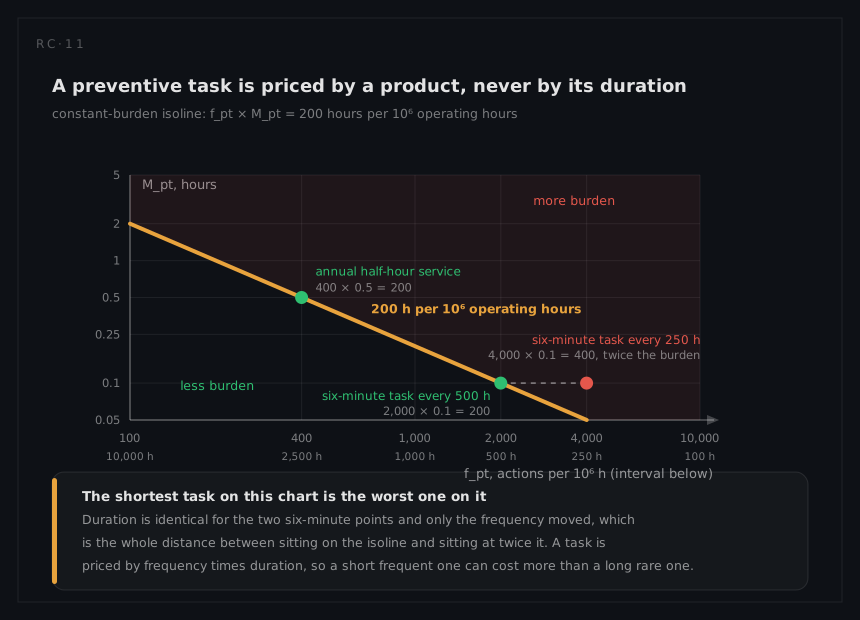
The measure that decides anything, though, is not Mpt on its own. Pair it with the rate at which the task recurs, fpt, the number of scheduled actions per unit of operating time, and the burden the task places on the system is the product:
preventive downtime per unit time = fpt × Mpt
A preventive task is priced by that product and never by its duration. The infusion pump fleet puts a scale on it. Each pump runs 2,500 hours a year and takes one half-hour annual service, so fpt = 400 actions per 10⁶ operating hours, Mpt = 0.5 h, and the burden is 400 × 0.5 = 200 hours per 10⁶ operating hours: 0.02% of the pump's operating time. Hold that burden fixed and ask what else buys it. A six-minute task, Mpt = 0.1 h, matches it only if it recurs no more often than every 500 operating hours, because 2,000 × 0.1 = 200. Schedule the same six-minute task every 250 hours instead and it costs 4,000 × 0.1 = 400 hours per 10⁶, twice the burden of a task five times its length. The short frequent task wins every comparison quoted in minutes per action and loses every ledger that counts hours per year.
One qualification keeps the product honest: it is downtime only when the task takes the system out of service. Work that fits a window the mission was not using costs labour and workshop capacity without costing availability, which is why availability's composition chapter argues for aggregating scheduled work into planned windows, and why the pump fleet's annual service is taken out of the biomedical department's capacity before the corrective queue is solved rather than queued inside it. Preventive work always lands in the man-hour ledger (MMH/OH); whether it lands in the downtime ledger is a scheduling decision, and the two are tracked separately.
Combining the streams: M̄ and MTBM
Corrective and preventive actions arrive as two streams into one maintenance organisation, and the quantities an availability model wants are properties of the sum rather than of either branch. Set the two side by side for the same pump, corrective at the fleet rate of 1,460 failures per 10⁶ hours and 0.75 hours of active repair, preventive at the annual service:
| Stream | Rate per 10⁶ operating hours | Mean time per action (h) | Downtime per 10⁶ operating hours (h) |
|---|---|---|---|
| Corrective | λ = 1,460 | M_ct = 0.75 | 1,095 |
| Preventive | fpt = 400 | M_pt = 0.50 | 200 |
| Combined | λ + fpt = 1,860 | M̄ = 0.696 | 1,295 |
The middle cell of the last row is the combined mean maintenance time, the rate-weighted average across the two streams:
M̄ = (λ × Mct + fpt × Mpt) / (λ + fpt)
M̄ = (1,460 × 0.75 + 400 × 0.50) / 1,860 = 1,295 / 1,860 = 0.696 h
This is the weighting argument of the λ-weighted rollup in the systems chapter applied across streams instead of across items: actions average in proportion to how often they occur. M̄ lands at 0.696 hours, far nearer the corrective 0.75 than the preventive 0.50, because corrective actions outnumber scheduled ones 3.65 to 1. The military handbooks write the quantity M̄ and call it the mean active maintenance time, active because it still excludes the logistics and administrative delays that turn it into MDT.
The denominator of that same fraction is the second quantity:
MTBM = 1 / (λ + fpt) = 10⁶ / 1,860 = 537.6 h
against an MTBF of 10⁶/1,460 = 685 hours, the figure the availability page for the same fleet computes from the identical rate. MTBF is the interval between failures, and availability needs the interval between down events: a scheduled service takes the system out of service exactly as effectively as a failure does. Putting MTBF where MTBM belongs credits this pump with 685 hours of uptime per interruption when it delivers 538, overstating the up-cycle by 27%. This ledger is deliberately restricted to the annual service. Add the two-year battery exchange that the preventive trade below also charges to the pump and fpt rises to 600 per 10⁶ hours, MTBM falls to 485 hours, and the same substitution overstates the up-cycle by 41% instead.
Both forms then run through their availability definitions from availability's foundations chapter:
Ai = MTBF / (MTBF + Mct) = 685 / (685 + 0.75) = 0.99891
Aa = MTBM / (MTBM + M̄) = 537.6 / (537.6 + 0.696) = 0.99871
Both figures assume ideal support: a repair channel available on demand, with no queue in front of it. The same fleet's queued reality is worked on the availability page, and the distance between the two is the distance between an inherent number and an operational one. The step from Ai to Aa is the smaller and the more explicable of the two: 2.73 hours of downtime per pump-year becomes 3.23, and the half hour between them is the service visit itself, arriving once. That is the entire content of the step from inherent to achieved availability: the maintenance policy's own downtime, added. Both terms the step is computed from, M̄ and MTBM, are owned here rather than in the availability topic, which states the formula and takes the numbers as given.
Two bookkeeping rules keep the arithmetic sound. λ and fpt must be expressed against the same clock, per operating hour above, but per calendar hour, per cycle or per kilometre wherever the maintenance interval is set that way; and both rates are per unit of uptime, which is what makes MTBM = 1 / (λ + fpt) an uptime interval that pairs correctly with M̄ in the availability ratio.
The preventive trade
The maintenance-action rate is a sum the programme controls from both ends, and the two ends move in opposite directions. Adding a preventive task raises λ + fpt immediately and by the full fpt. It lowers λ only if the mode the task targets is one scheduled work can pre-empt, and then only by the fraction the task actually catches. A preventive programme is therefore a trade, priced by comparing the corrective downtime it removes against the scheduled downtime it adds:
Δλ × Mct > Δfpt × Mpt
The pump's battery is the case where the trade wins clearly. The rate that enters as Δλ is the battery's 800 per 10⁶ operating hours, which is the two handling events a pump-year its fitted Weibull produces on a seven-month cycle, counted on the pump's own running clock. The policy change worked on the availability page (moving replacement from the characteristic life to the B10 age of the fitted battery distribution) converts roughly 560 of the fleet's 1,750 annual unscheduled arrivals into planned exchanges. That is 2 × 0.75 = 1.5 hours of corrective downtime removed per pump-year in exchange for one scheduled exchange a year, so the inequality prices the exchange directly:
Mpt < (Δλ × Mct) / Δfpt = 1.5 / 0.5 = 3.0 h
The exchange rate rises from 0.5 to 1 per pump-year rather than from nothing to one, so the denominator is the half-action the policy adds, not the whole task.
That is comfortable for a task whose corrective equivalent is 45 minutes on the same bench. The action ledger moves with it: preventive actions rise from 1.5 to 2, and the total falls from 5.15 to 3.65 per pump-year. The total fell only because the targeted mode is frequent and genuinely ageing, β = 3.4 on the reliability page for the same fleet.
That combination is the exception rather than the rule. Where a mode has no wear-out region for scheduled work to exploit, Δλ is zero at every interval, the inequality can never be satisfied, and fpt × Mpt is pure loss, before counting the infant-mortality failures an intrusive task introduces. That is the reliability-centred maintenance finding of the design chapter restated as arithmetic, and it is why RCM tests whether a task is applicable at all before it argues about intervals.
The same arithmetic sets a reporting trap, because M̄ is a weighted mean and short frequent tasks pull it down. Replace the pump's annual half hour with the six-minute task every 250 hours, fpt = 4,000 per 10⁶ hours:
M̄ = (1,460 × 0.75 + 4,000 × 0.10) / 5,460 = 1,495 / 5,460 = 0.274 h
MTBM = 10⁶ / 5,460 = 183.2 h
Aa = 183.2 / (183.2 + 0.274) = 0.99851
M̄ has fallen 61%, from 0.696 hours to 0.274, while downtime has risen from 3.23 to 3.73 hours per pump-year. M̄ falling is evidence of nothing on its own: it is one factor of a product, and the quantity that decides availability is the ledger's last column, the sum of rate times time over both streams. A maintainability report showing M̄ improving while MTBM shortens faster is describing a programme that bought downtime.
Where the numbers go next: M̄ and MTBM feed the achieved and operational availability formulas of availability's foundations chapter, the second of which writes Ao = MTBM / (MTBM + MDT) with the same denominator and full downtime in place of M̄. The combined action rate λ + fpt is what shared-channel models consume, and both pump pages spend it: the maintainability page routes both streams through one biomedical department, and the availability page adds 2,190 × 0.75 = 1,642 corrective hours to 600 × 0.5 = 300 preventive hours to size the channel. Mct alone continues to feed the failure-rate-weighted rollup of the systems chapter, which is a corrective-only calculation and should be labelled as one wherever it is quoted beside an availability number.
Estimating, predicting, demonstrating
Three different evidence sources feed the same measures, in programme order. Prediction comes first: while the design is on paper, elemental task times are estimated from the design's features (access, fasteners, test resolution, module weight) using the tabulated and scoring methods of the MIL-HDBK-472 lineage, rolled up per failure mode and weighted by the predicted failure rates. The output is a predicted MTTR and percentile per unit and per system, and its honesty depends on two inputs the maintainability engineer does not own: the failure-rate weights and the claimed fault-isolation coverage.
Demonstration converts the prediction into evidence on real hardware: a sample of faults is physically inserted or simulated, technicians of the specified skill level repair them using the specified documentation and tools, and the observed times are tested statistically against the requirement (the MIL-STD-471 lineage catalogues the sampling plans and accept/reject mathematics, built around the lognormal assumption). The classic demonstration failure modes are selection bias in the fault sample (only the easy faults get inserted) and condition drift (an engineer hovering behind the technician is not a stated condition).
Field measurement is the final authority and the messiest: real event logs mix active time with logistics and administrative delay, clocks start and stop inconsistently, and multiple-technician actions blur elapsed time against man-hours. The working rules: define the clocks before collecting (what starts MTTR, what starts MDT), record man-hours separately from elapsed time, and keep level-of-repair boundaries explicit so bench times and flight-line times never average together. Cleanly collected, field repair data closes the loop exactly as failure data does for reliability: it recalibrates the predictions, exposes the ambiguity groups the testability analysis overpromised on, and hands FRACAS its maintainability-flavoured findings.