

A system's maintainability is not the average of its parts' repair times, any more than its reliability is the average of its parts' lives. Repair times compose through the failure rates that trigger them, through the diagnostic resolution that scopes them, and through the maintenance organisation that executes them. This chapter covers the composition rules: the failure-rate-weighted rollup, the ambiguity arithmetic that couples maintainability to testability, the level-of-repair structure, and what repair speed does inside availability models.
The failure-rate-weighted rollup
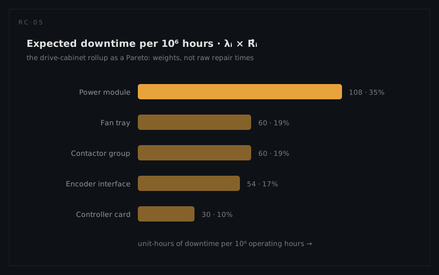
The system-level mean corrective time is the mean over repair events, and events arrive in proportion to failure rates. With item failure rates λᵢ and item mean repair times R̂ᵢ:
MTTRsys = Σ(λᵢ × R̂ᵢ) / Σλᵢ
a failure-rate-weighted average, standard in the military handbooks since the discipline's founding. The weighting is the whole insight: a slow repair on a rare item may cost less downtime than a quick repair on a frequent one, and no unweighted average reveals that.
A worked rollup on an invented example, a motor-drive cabinet with five replaceable units:
| Unit | λ (per 10⁶ h) | Mean repair R̂ᵢ (h) | λᵢ × R̂ᵢ | Share of expected downtime |
|---|---|---|---|---|
| Power module | 120 | 0.9 | 108 | 35% |
| Fan tray | 200 | 0.3 | 60 | 19% |
| Contactor group | 25 | 2.4 | 60 | 19% |
| Encoder interface | 45 | 1.2 | 54 | 17% |
| Controller card | 60 | 0.5 | 30 | 10% |
| Cabinet | 450 | MTTR = 312/450 = 0.69 h | 312 | 100% |
The cabinet's MTTR is 0.69 hours (about 42 minutes), and the table's last column is the improvement agenda: the power module drives over a third of expected downtime despite a moderate repair time, because it fails often. Halving the contactor group's 2.4-hour repair (the worst raw time) buys less than shaving twenty minutes off the power module's. This λ-weighted Pareto is the maintainability twin of the failure-rate Pareto in the reliability systems chapter, and the two should be read together: the same item list, two different orderings, one shared improvement budget.
The rollup also exposes the analysis's dependencies. The weights come from the reliability prediction, so a stale prediction quietly corrupts the maintainability numbers; and the R̂ᵢ are conditional on the diagnostic and access assumptions of the next section. The rollup is arithmetic; its inputs are the engineering.
Ambiguity: where diagnosis multiplies repair
The elemental times of the foundations chapter assumed the failed unit is known. Whether it is known is the testability analysis's output: fault isolation rate says what fraction of failures the built-in test resolves to one unit, and to how large an ambiguity group it resolves the rest. Ambiguity converts directly into time. If the test names a three-card group and the technician swaps sequentially, the expected number of swaps to hit the faulty card is two (equal priors), so a nominal 15-minute interchange becomes 30 minutes of swapping plus a second checkout cycle, and the spares ledger is charged for good cards pulled from service, a cost that surfaces later as no-fault-found returns.
The system-level consequence: a design's effective repair time is a mixture across isolation outcomes. A unit with a 20-minute isolated-repair time, 80% single-unit isolation, and a three-unit ambiguity group otherwise does not have a 20-minute repair; it has roughly 20 minutes four times out of five and 50-plus minutes otherwise, and the percentile commitments feel the second branch hard. This is why maintainability reviews interrogate the isolation claims behind every predicted repair time, and why the FMEA-to-testability chain (which failure modes are detectable, by what test, to what resolution) sits upstream of every honest MTTR prediction.
Levels of repair
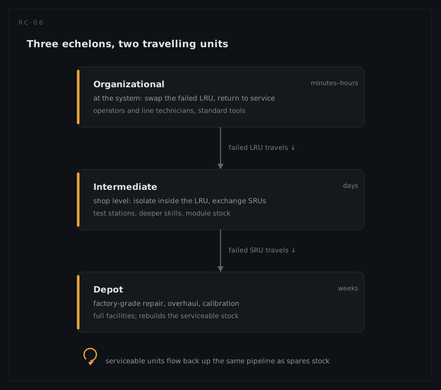
Maintenance is organised in echelons, classically three: organisational (at the system, by its operators or line technicians: swap and go), intermediate (a nearby shop with test equipment: diagnose and exchange modules), and depot (the factory-grade facility: full repair, overhaul, calibration). The design's replaceable-unit structure maps onto the echelons: LRUs (line-replaceable units) are sized and interfaced for fast exchange at organisational level; SRUs (shop-replaceable units) are the boards and modules exchanged inside an LRU at the shop levels.
The partition is a design decision with system-wide consequences, and each choice trades four currencies:
| Choice | Buys | Costs |
|---|---|---|
| Bigger LRUs (swap whole drawer) | Fast restoration, low skill at the line | Expensive spares pipeline, more no-fault-found volume |
| Smaller LRUs (swap one card) | Cheap spares, precise replacement | Needs sharper isolation and more line time |
| More capability at lower echelons | Short turnaround loops | Duplicated test equipment and skills at every site |
| Centralised repair | Efficient facilities, consistent quality | Long pipelines, deeper spares float to cover them |
Where each repair should happen is an economic and operational optimisation, not a convention, and it is exactly the question level of repair analysis formalises: for every repairable item, compare repair-at-each-echelon against discard, under the costs of spares, transport, test equipment, and downtime. The maintainability numbers of this topic are its inputs; the maintenance concept it outputs then becomes the stated conditions under which every MTTR in the specification is defined. The loop closes: repair times assume an echelon structure, and the echelon structure is chosen using the repair times.
Repair speed inside availability models
Once systems are repairable, maintainability stops being a bookkeeping annex and becomes a model parameter with leverage. Three effects dominate:
- The availability balance. For a single repairable item, steady-state availability is MTBF/(MTBF + MTTR): repair time enters on equal footing with failure time, and the operational form substitutes full downtime (MDT) for MTTR, which is how a support-system delay becomes an availability loss indistinguishable from unreliability.
- Redundancy lives on repair. A redundant pair fails as a system only when the second unit fails while the first is still down, so the exposure window is the repair time. Halve the repair time and the pair's system failure rate roughly halves; let a failed channel linger undetected (a latent failure, the detection-interval problem) and the redundancy silently degrades to a single string. Repairable-redundancy arithmetic is where RBD availability modelling earns its keep, and its most sensitive inputs are restoration times and detection intervals, not the failure rates.
- Shared crews queue. When one crew or one test stand serves many systems, repairs queue behind each other and effective downtime exceeds every individual repair time. Staffing and support-equipment decisions are therefore availability decisions, sized with queueing or simulation arguments rather than single-repair means.
All three effects meet in the availability topic, which builds the repairable-system mathematics on top of this chapter and reliability's; it precedes this one in the Concepts row (Availability). What matters here is the direction of dependence: availability models are only as honest as the restoration times fed into them, and restoration times are only as honest as the diagnosis, access, and echelon assumptions built into the design.