

Everything quantitative in reliability engineering rests on one idea: treat time to failure as a random variable. A single unit's failure time cannot be predicted, but a population's failure behaviour follows a distribution, and once that distribution is named, everything else (survival probabilities, failure rates, expected lives, warranty exposure, spares demand) is arithmetic on it. This chapter builds that machinery in the order a practitioner actually needs it: the four functions that describe failure, the point measures quoted in requirements, the distributions that model real hardware, and the physical pictures (bathtub, overstress versus wear-out, load versus strength) that tell you which mathematics applies.
Notation used in this topic
| Symbol | Reads as | Meaning |
|---|---|---|
| R(t) | reliability function | probability of surviving beyond time t |
| F(t) | cumulative distribution | fraction failed by t, equal to 1 − R(t) |
| f(t) | density | where on the time axis failures concentrate |
| h(t) | hazard rate | instantaneous failure rate among survivors, f(t)/R(t) |
| H(t) | cumulative hazard | integral of h(t), giving R(t) = e^(−H(t)) |
| λ | lambda | failure rate, usually assumed constant |
| β | beta | Weibull shape parameter: the failure-regime diagnosis |
| η | eta | Weibull characteristic life, the 63.2% point |
| Γ(·) | gamma function | the factor that turns a Weibull characteristic life into a mean life |
| MTBF, MTTF | mean time between failures (repairable), mean time to failure (non-repairable) | |
| FIT | failures in time | one failure per 10⁹ device-hours |
tp | life percentile | the age by which a fraction p of the population has failed |
| B10 | B-life | time by which 10% of the population has failed |
Every abbreviation used anywhere in RAMS Core is defined in the glossary.
The four functions of failure
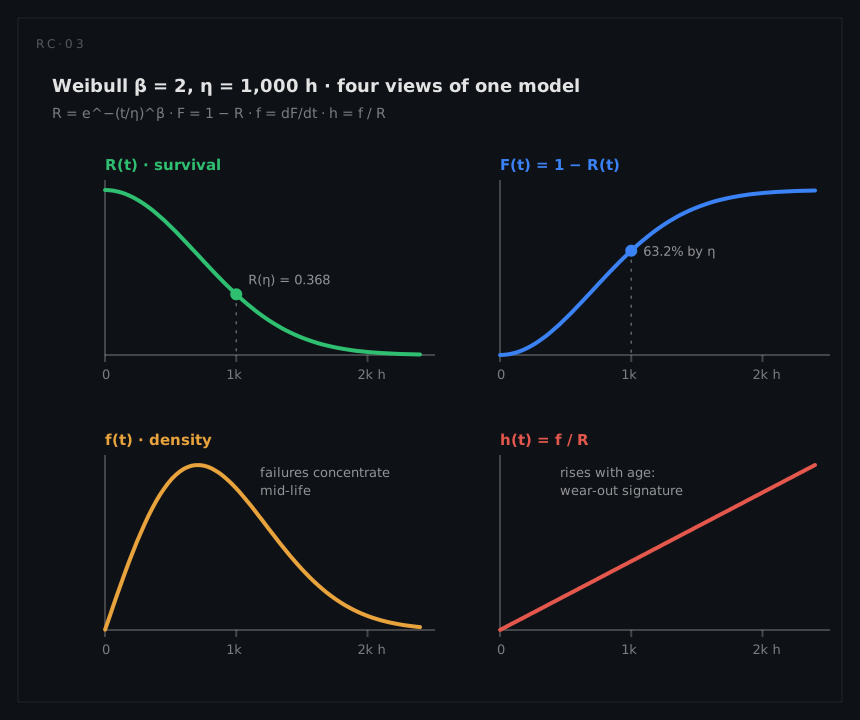
Let T be the time to failure of an item. Four equivalent functions describe it, and fluency in moving between them is the core skill of the discipline:
- The reliability function
R(t) = P(T > t): the probability of surviving beyond t. It starts at 1 and can only fall. - The cumulative distribution
F(t) = P(T ≤ t) = 1 − R(t): the fraction of the population failed by t. - The density
f(t) = dF/dt: where on the time axis failures concentrate. - The hazard rate
h(t) = f(t)/R(t): the instantaneous failure rate among survivors. This is the conditional view: given that the item has lived to t, how likely is it to fail in the next instant?
The hazard deserves the emphasis it gets, because it is the function with physical meaning. A decreasing hazard says the population is being purged of weak units; a constant hazard says failures arrive at random with no memory; an increasing hazard says something is being consumed: material, lubricant, insulation, life. Integrating the hazard gives the cumulative hazard H(t) = ∫h(u)du, and the single most useful identity in the subject:
R(t) = e^(−H(t))
Every named life distribution is just a choice of hazard shape pushed through this identity. From R(t) also comes the mean life of a non-repairable item, MTTF = ∫R(t)dt over all time: the area under the survival curve.
Point measures and their units
Requirements and datasheets compress the functions above into single numbers. Each is legitimate; each also loses information, and most reliability misunderstandings start with a point measure quoted outside its context.
| Measure | What it is | Unit conventions | The trap |
|---|---|---|---|
| Failure rate λ | Hazard rate, usually assumed constant | failures per 10⁶ h; FIT = failures per 10⁹ device-hours | Only meaningful while the constant-rate assumption holds |
| MTBF | Mean time between failures of a repairable item | hours | Not a life; not a guarantee; ~63% of an exponential population fails before it |
| MTTF | Mean time to failure of a non-repairable item | hours | Averages hide shape: two very different distributions can share an MTTF |
| B₁₀ life | Time by which 10% of the population has failed (B₅, B₁ likewise) | hours, cycles, km | Says nothing about the other 90% without the distribution |
Mission reliability R(tm) | Probability of completing a mission of length tm | dimensionless | Meaningless without the mission profile attached |
| MTTR | Mean time to repair: a maintainability measure | hours | Belongs in the availability equation, not the reliability one |
Three of these repay a closer look. MTBF versus MTTF is not pedantry: the classic definitions (MIL-STD-721C) reserve MTBF for repairable items and MTTF for non-repairable ones, and quoting an MTBF for a one-shot or throwaway item is a category error that usually signals a copied number. FIT arithmetic is a unit convention worth internalising: 1 FIT is one failure per 10⁹ device-hours, so a component at 100 FIT has λ = 10⁻⁷ per hour and an MTBF (if constant-rate and repairable) of 10⁷ hours. And the MTBF-is-not-a-lifetime trap is the industry's most persistent: an electronic unit with a 200,000-hour MTBF is not expected to last 23 years; it is expected to fail at a rate of one per 200,000 unit-hours while it is within its useful life, which may be a tenth of that. The rate describes the plateau of the bathtub curve, not the length of the tub.
Percentile lives (B-lives) are often the more honest requirement currency, especially for wear-out-driven hardware: "B₁₀ ≥ 15,000 hours" pins the early tail of the distribution, which is what warranty exposure and safety cases actually care about, in a way no mean ever can.
Life distributions
Four continuous distributions and two discrete ones cover almost all practical reliability work:
| Distribution | Parameters | Hazard behaviour | Where it earns its keep |
|---|---|---|---|
| Exponential | λ | Constant (the only distribution with this property) | Useful-life electronics; systems whose failures are externally driven; the default of the prediction handbooks |
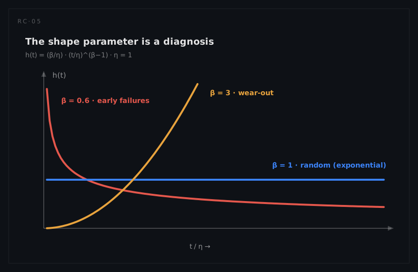
| Weibull | shape β, scale η | Falling (β < 1), constant (β = 1), rising (β > 1) | The general-purpose life model; β diagnoses the failure regime, η is the characteristic life |
| Lognormal | μ, σ | Rises then falls | Degradation processes that multiply (fatigue crack growth, corrosion, some semiconductor mechanisms); also repair times |
| Normal | μ, σ | Rising | Tightly clustered wear-out (filament life, some mechanical wear); strength and load scatter in interference models |
| Binomial | n, p | per-demand | One-shot devices: the probability of k successes in n firings |
| Poisson | λt | per-interval | Counts of failures in a fixed exposure; the arithmetic behind spares provisioning and standby redundancy |
The exponential distribution, R(t) = e^(−λt), dominates the field's history because of its memoryless property: a survivor is statistically as good as new, so the failure rate of a fleet is constant regardless of age mix. That single assumption makes system arithmetic linear (rates add), which is why the prediction handbooks and most availability models run on it. It is an assumption to be earned, not presumed: it holds well for complex electronics in their useful life and fails badly for anything that wears.
The Weibull distribution, R(t) = e^(−(t/η)^β), is the practitioner's workhorse precisely because it does not presume. The shape parameter β is a regime diagnosis read straight from data: β < 1 flags infant mortality (improve the process or screen), β ≈ 1 flags randomness (add margin or redundancy; preventive replacement is useless), β > 1 flags wear-out (schedule replacement before the hazard climbs). The scale parameter η is the characteristic life, and at β = 1 the Weibull collapses exactly to the exponential with η = 1/λ. Fitting β and η from test or field data is the subject of life data analysis, and the fitted parameters are what the design-side analyses should be fed. The subsection below states the three formulas that turn a fitted pair into hazards, percentiles and mean lives, and works them end to end on one item.
The Weibull working formulas
A fitted pair of parameters is not two facts about an item; it is the item's entire life. Three formulas convert that pair into everything a programme quotes: every hazard, percentile and mean life given for a Weibull item on the industry example pages comes from these three, applied to R(t) = e^(−(t/η)^β). All three are written for the two-parameter Weibull, γ = 0, which is what every fit in RAMS Core uses; a fitted threshold shifts all three by γ.
The hazard rate is the shape's operational face: the instantaneous risk carried by a survivor of age t.
h(t) = (β/η)(t/η)^(β−1)
The life percentile tp, the age by which a fraction p of the population has failed, comes from inverting the reliability function.
tp = η(−ln(1 − p))^(1/β)
B10 is this formula at p = 0.10, where −ln(0.9) = 0.10536; the median is p = 0.50, where −ln(0.5) = 0.69315.
The mean life is the area under the survival curve, and for the Weibull that integral closes into a gamma function.
MTTF = η · Γ(1 + 1/β)
Two corollaries of the hazard formula are worth memorising. Setting t = η gives h(η) = β/η, so the characteristic life is also the age at which the hazard equals shape divided by scale. And the growth of the hazard per doubling of age depends on β alone, not on η and not on where the doubling starts:
h(2t)/h(t) = 2^(β−1)
which is 1.00 for any constant-rate item at any age, 1.52 at β = 1.6, 1.87 at β = 1.9 and 5.28 at β = 3.4. That ratio, rather than the rate itself, is what a maintenance interval is argued from.
η is the 63.2% point, whatever β is. Put t = η into R(t) = e^(−(t/η)^β): the bracket becomes 1 for every shape, so R(η) = e^(−1) = 0.3679 and F(η) = 0.6321. The characteristic life is therefore not a mean, not a median and not a safe life; it is the age by which 63.2% of the population is gone. A replacement interval set at η is an interval set at that percentile, which is why the infusion-pump battery replaced at its characteristic life reaches the bench with 63% of the population already failed.
The gamma function is the only part of the three formulas a calculator keypad will not evaluate, so the values for the shapes this book uses are tabulated here to four significant figures, enough to reproduce every Weibull mean life quoted in RAMS Core.
| β | 1 + 1/β | Γ(1 + 1/β) | Where the shape appears |
|---|---|---|---|
| 1.0 | 2.0000 | 1.0000 | The exponential special case, where MTTF = η = 1/λ |
| 1.4 | 1.7143 | 0.9114 | Brake actuator |
| 1.6 | 1.6250 | 0.8966 | Infusion pump plunger drive |
| 1.9 | 1.5263 | 0.8874 | Level-crossing barrier drive |
| 2.0 | 1.5000 | 0.8862 | Generator drive, carried as the counterfactual shape |
| 2.2 | 1.4545 | 0.8856 | Spacecraft reaction wheel |
| 3.1 | 1.3226 | 0.8943 | Compressor hot section |
| 3.4 | 1.2941 | 0.8984 | Infusion pump battery |
The third column barely moves, and that is itself a working fact. For any β ≥ 1 the argument 1 + 1/β lies between 1 and 2, where the gamma function dips to a minimum of 0.8856 at β ≈ 2.17 and returns to 1.0000 at both ends, so the mean life of any Weibull item that is not in infant mortality sits between 88.6% and 100% of its characteristic life. Below β = 1 the relation inverts and is unbounded: at β = 0.5, Γ(3) = 2 and the mean is twice η, because a falling hazard leaves a long-lived remnant population. For the wear-out shapes that fill the table, η is always a fair estimate of the mean and the mean is never an estimate of a percentile, and the next few lines show how far apart those two readings are on one real item.
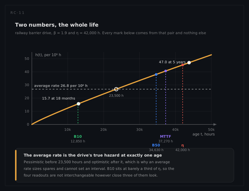
One pair of parameters, four answers. Take the barrier drive fitted from six years of field returns on the level-crossing page: β = 1.9, η = 42,000 hours, and no other input. The hazard scale is β/η = 1.9 / 42,000 = 4.524 × 10⁻⁵ per hour, which by the corollary above is the hazard at the characteristic life itself, 45.2 per 10⁶ hours. Evaluated at two ages a maintenance planner chooses between, eighteen months of continuous service and five years:
h(13,000) = 4.524 × 10⁻⁵ × (13,000 / 42,000)^0.9 = 4.524 × 10⁻⁵ × 0.3480 = 1.57 × 10⁻⁵ per hour
h(43,800) = 4.524 × 10⁻⁵ × (43,800 / 42,000)^0.9 = 4.524 × 10⁻⁵ × 1.0385 = 4.70 × 10⁻⁵ per hour
15.7 per 10⁶ hours against 47.0, the same drive at two ages, and the whole factor of 2.98 between them is (43,800 / 13,000)^0.9. The percentiles come from the second formula:
B10 = 42,000 × (0.10536)^(1/1.9) = 42,000 × 0.3059 = 12,850 h
B50 = 42,000 × (0.69315)^(1/1.9) = 42,000 × 0.8246 = 34,630 h
and the mean from the third, reading Γ(1.5263) = 0.8874 off the table:
MTTF = 42,000 × 0.8874 = 37,270 h
That mean is quoted as 37,300 wherever this drive appears elsewhere, rounded to three figures. Its reciprocal is the item's average rate across its whole life:
λ̄ = 1 / (η · Γ(1 + 1/β)) = 1 / 37,270 = 26.8 per 10⁶ h
That last figure is legitimate for sizing spares and labour and illegitimate as a hazard rate: it lies between the 15.7 and the 47.0 computed above and equals the drive's true hazard at exactly one age, near 23,500 hours. Two numbers fix the whole life. A tenth of the drives are gone by 12,850 hours, half by 34,630, the average is 37,270, the risk to a survivor nearly triples across the interval a policy has to choose within, and every one of those figures is arithmetic on β = 1.9 and η = 42,000 with nothing else supplied.
β and the three bathtub regions. The mapping is one to one, and the last column is what converts a fitted shape into a maintenance decision:
| Fitted β | Hazard | Bathtub region | A survivor of age t, against a new unit |
|---|---|---|---|
| β < 1 | Falling | Early failures | Better: it has passed the weeding, so fitting a new unit raises the risk. This is the entire argument for burn-in |
| β = 1 | Constant | Useful life | Identical: the memoryless property. Replacement changes nothing, at any age |
| β > 1 | Rising | Wear-out | Worse: damage has accumulated, so replacement lowers the risk. This is what makes an interval worth setting |
How far above 1 the shape sits matters as much as the direction, because β controls the spread. The coefficient of variation of a Weibull life falls as β rises: 0.640 at β = 1.6, 0.547 at β = 1.9 and 0.325 at β = 3.4. A wide population is a population in which a life limit retires a great deal of good hardware to catch the early tail, and a tight one is where a limit is efficient. That is why the barrier drive at β = 1.9 earns an age-replacement task at its B10 of 12,850 hours, written as 13,000 in the task itself, and why the case is much weaker for the plunger drive at β = 1.6.
One caution applies to reading a fitted β at all. A mixture of mechanisms with different shapes flattens towards an apparent β near 1, so a straight line on a probability plot is evidence about the population that was fitted and not about any mechanism inside it; the infusion pump page works that trap in full.
One-shot devices (squibs, fuzes, airbag igniters, deployment mechanisms) break the time-based frame entirely: their reliability is a probability per demand, estimated from binomial trials, and their "life" question (does storage age degrade the per-demand probability?) is a separate, sampled-surveillance problem.
The bathtub curve and its limits
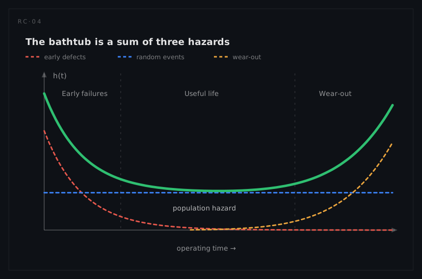
Plot the hazard rate of a large, mixed population of hardware over its whole life and the classic shape appears: a falling early region, a long flat middle, a rising tail.
| Region | Hazard | Dominant causes | Effective countermeasures |
|---|---|---|---|
| Early failures (infant mortality) | Falling | Manufacturing defects, workmanship escapes, damaged parts, installation errors | Process control, inspection, environmental stress screening |
| Useful life | Roughly constant | Residual defects and externally induced events (transients, mishandling, environment) | Margin, derating, protection, redundancy |
| Wear-out | Rising | Fatigue, wear, corrosion, insulation ageing, electromigration | Preventive replacement, life-limiting, redesign of the weak mechanism |
The curve is genuinely useful as a vocabulary: it names the three hazard regimes, maps them onto Weibull β ranges, and explains why the countermeasure must match the regime (screening does nothing for wear-out; preventive replacement does nothing for random failures). But treat it as a composite picture of a population, not a law of nature for a device. Individual failure mechanisms follow their own single-regime hazards, and the published critique of the model (Klutke and colleagues' "critical look" in the IEEE Transactions on Reliability) shows that real populations rarely trace the idealised tub; in particular, the early-life hazard of well-made products is often not decreasing at all, which undercuts naive burn-in justifications. The practical reading: use the bathtub to ask which regime each mechanism of your design lives in, and demand data (a fitted β, a screening fallout trend) before spending money on regime-specific countermeasures.
Overstress and wear-out
Beneath the statistics, hardware fails for physical reasons, and nearly all of them sort into two classes. Overstress failures happen when an applied load exceeds the item's strength at that moment: electrical transient over a junction's rating, mechanical shock past a bracket's yield, thermal excursion past a material limit. They are sudden, and their statistics follow the loads: if extreme loads arrive at random, overstress failures inherit a roughly constant hazard. Wear-out failures happen when strength degrades below the routine load: fatigue accumulates cycle by cycle, corrosion thins a section, electromigration voids a conductor, insulation ages, contacts wear. They are progressive, and their statistics show rising hazards and finite lives.
| Class | Mechanism examples | Statistical signature | Design lever |
|---|---|---|---|
| Overstress | Dielectric breakdown from transients, ESD damage, fracture under shock, thermal runaway | Hazard tracks the load environment; often β ≈ 1 | Margin: derating, protection circuits, load isolation |
| Wear-out | Fatigue, wear, corrosion, creep, electromigration, solder-joint thermal fatigue, battery ageing | Rising hazard, β > 1, finite characteristic life | Slow the mechanism (stress, temperature), or life-limit and replace |
The class distinction is what connects the physics to the mathematics: it tells you which distribution to expect before any data exist, and it tells you which design lever can work. It is also the intellectual basis of physics-of-failure practice, which models the dominant mechanism directly (a fatigue law, an electromigration model, an ageing model) instead of wrapping everything in one generic rate. The prediction topic's foundations chapter covers where handbook rates and physics-of-failure models each belong.
Load, strength, and margin
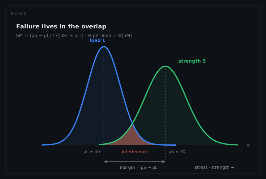
Why does one design fail at ten times the rate of another built to the same nominal stress ratio? The interference picture answers it. Treat the applied load L and the item's strength S as random variables: load varies with usage, environment, and events; strength varies with materials, tolerances, and manufacturing. Failure occurs when L > S, and the failure probability is governed by the overlap of the two distributions.
For normally distributed load and strength, the standard result condenses the overlap into a single number, the safety margin:
SM = (μS − μL) / √(σS² + σL²)
the separation of the means measured in units of the combined scatter. Reliability per load application is Φ(SM), the standard normal probability below that margin. The insight worth carrying is that variance is as important as mean: widening the gap between mean strength and mean load helps, but so does narrowing either distribution, and a traditional safety factor (ratio of nominal strength to nominal load) is blind to the scatter entirely. Two lessons follow directly. First, derating works because it shifts μL down wholesale, buying margin against the whole load distribution at the cost of using a bigger part. Second, quality control works on reliability through σS: tightening process variation narrows the strength distribution and pulls the weak tail out of the interference zone. Wear-out joins this picture as strength degradation: S drifts downward with age, the overlap grows, and the hazard rises, which is exactly the β > 1 signature seen in the data.
Estimating from data
Everything above assumed the distribution was known. In practice it is estimated, from test or field data, and the estimate carries uncertainty that honest engineering must quote.
For constant-rate items the machinery is compact. Observe r failures in T accumulated unit-hours and the point estimate is λ̂ = r/T. Its uncertainty comes from the chi-square distribution: for a time-truncated observation, the upper confidence bound on the rate at confidence level C is
λupper = χ²(C; 2r + 2) / 2T
with the matching lower bound on MTBF being 2T/χ². A worked instance shows why the bound matters more than the estimate. Suppose a fleet accumulates 100,000 hours with 5 failures: λ̂ = 50 failures per 10⁶ hours, MTBF estimate 20,000 hours. At 90% confidence, χ²(0.90; 12) = 18.55, so λ could be as high as 92.7 per 10⁶ hours and the demonstrated MTBF is only 10,780 hours: barely half the point estimate. Requirements phrased as "demonstrate 20,000 h MTBF at 90% confidence" are therefore asking for far more test time than 20,000 hours, which is the arithmetic behind every reliability demonstration test plan.
The zero-failure special case is the success-run formula. To demonstrate reliability R per mission at confidence C with no failures allowed, the required number of independent trials is
n = ln(1 − C) / ln(R)
which prices out demonstration testing brutally fast: showing 99% mission reliability at 90% confidence takes 230 failure-free trials, and every "nine" added to R multiplies the bill by roughly ten. This single formula explains much of reliability programme design: pure end-of-programme demonstration is unaffordable for high targets, so real programmes buy their evidence earlier and cheaper, through analysis, margin, growth testing, and field surveillance instead.
Field and test data rarely come clean: most units are still alive when the analysis runs (right-censored), some fail between inspections (interval-censored). Estimation that ignores censoring is biased, always optimistically on the failed units and pessimistically on the fleet. The full treatment (median-rank plotting, maximum likelihood, confidence bounds on Weibull parameters) belongs to life data analysis, and the short rule here is: never fit a life distribution to failure times alone while discarding the survivors, because the survivors are most of the information.