

Notation used in this topic
| Symbol | Reads as | Meaning |
|---|---|---|
| λ | lambda | failure rate: expected failures per unit of operating time |
λp | lambda-p | the rate a part model returns for one part under its own conditions |
λb | lambda-b | base failure rate of a part class at the handbook's reference condition (written λB in the K-factor lineages) |
λg | lambda-g | generic failure rate a part class carries in the parts count procedure |
λEQUIP | the equipment rate the parts count sum produces | |
λgoal | the rate budget an allocated MTBF converts into, and what the prediction is compared against | |
λoperating, λdormant, λcalendar | one box's rate while energised, while switched off, and averaged over the calendar | |
| λᵢ, tᵢ | the rate and the duration of mission phase i | |
| MTBF, MTTF | mean time between failures (repairable), mean time to failure (non-repairable) | |
| MTTR, A | mean time to repair, availability | the maintainability half of the availability equation, and the uptime fraction the pair combines into |
| FIT | failures in time | one failure per 10⁹ operating hours, so 1,000 FIT is one failure per 10⁶ hours |
| R(t) | reliability function | probability of surviving to time t |
| R(T, τ) | conditional reliability | probability of surviving a further mission of duration τ given survival to age T |
| π_T, π_Q, π_E, π_L | pi-T, pi-Q, pi-E, pi-L | the factors present in nearly every 217F model: temperature, quality, environment, learning |
| π_A, π_R, π_S, π_C | the part-category factors: application, power rating, electrical stress, construction | |
KE, KS | K-E, K-S | the K-factor lineages' environment factor and combined stress-and-temperature factor |
| C₁, C₂ | C-one, C-two | the microcircuit model's die-complexity and package-complexity coefficients |
Ea, k | activation energy, Boltzmann constant | the Arrhenius pair behind π_T, with k = 8.617×10⁻⁵ eV/K |
TJ, TC | junction temperature, case temperature | the part temperatures the stress models run on; TJ enters the Arrhenius factor in kelvin |
θJC, θJA, θCA | theta-JC, theta-JA, theta-CA | thermal resistance junction-to-case, junction-to-ambient, and case-to-ambient |
| P | power dissipated in the part | |
| N, Nᵢ | quantity of a part class in the inventory; in the event-driven form, the number of cycles | |
| p | probability of failure per event, for mechanisms that count cycles rather than hours | |
| d | duty cycle | the fraction of the calendar the equipment is energised |
PF | per-demand failure probability of a one-shot device | |
| Cm, α, β | criticality number, mode ratio, conditional probability | the MIL-STD-1629A criticality arithmetic that consumes the predicted rate |
| B₁₀ | B-ten life | the time by which 10% of a population has failed: an input to the mechanical models |
Every abbreviation used anywhere in RAMS Core is defined in the glossary.
The quantities and their units
The primary quantity is the failure rate λ, the expected number of failures per unit of operating time. MIL-HDBK-217F expresses every rate in failures per 10⁶ hours; the telecom and European traditions (Telcordia, IEC, Siemens) work in FIT, failures per 10⁹ hours. Unit confusion between the two conventions is a classic audit finding, so keep the conversion at hand:
| Quantity | Definition | Conversion |
|---|---|---|
| λ (217F convention) | failures per 10⁶ operating hours | 1 f/10⁶ h = 1,000 FIT |
| FIT (Telcordia / IEC convention) | failures per 10⁹ operating hours | 1 FIT = 0.001 f/10⁶ h |
| MTBF | mean operating time between failures | MTBF = 1/λ (constant-rate assumption) |
| R(t) | probability of surviving to time t | R(t) = e^(−λt) |
Under the constant-rate assumption, MTBF is nothing more mysterious than the reciprocal of λ. A system predicting 20 f/10⁶ h has an MTBF of 50,000 hours, and, less intuitively, only a 37% chance of actually reaching 50,000 hours without failure, because e^(−1) ≈ 0.368. An MTBF is a mean, not a guarantee, and for exponential lifetimes the mean sits well past the median.
The mean-time vocabulary deserves one moment of pedantry, because practice is sloppy with it. MTBF: mean time between failures, belongs to repairable items, where repair restores operation and several failures over the life are expected. MTTF: mean time to failure, belongs to non-repairable items (an orbiting satellite is replaced, not repaired). For a non-repairable item the two coincide numerically, which is why the terms get used interchangeably; but writing "MTBF" on a one-way device quietly implies a repair concept that does not exist, and a careful report says which it means. Downstream, the pair MTBF and MTTR (mean time to repair, from the maintainability prediction) combine into steady-state availability, A = MTBF / (MTBF + MTTR), which is the quantity redundancy and uptime arguments actually run on.
The constant-rate assumption and what it buys
The exponential distribution is the only lifetime distribution with a constant hazard rate: no memory, no ageing. Assuming it buys the method its entire algebra: failure rates of series elements add, so a system's rate is the sum of its parts' rates and the roll-up is a single pass of arithmetic up the product structure. It also defines the method's blind spots. A prediction cannot tell you when wear-out begins, cannot see batch-dependent infant mortality, and cannot represent a part whose risk grows with cycles rather than hours. Those questions belong to life-data analysis and physics-of-failure methods, not to the handbook.
Two refinements keep the assumption honest rather than naive. First, real systems mix behaviours: most electronics sit close to a constant rate through their useful life, mechanical items carry rising, age-driven rates (fatigue, wear, corrosion, creep), and single-use devices are not time-governed at all. The constant-rate framework survives this mix better than it looks like it should, in a maintained system whose items are replaced at failure and retired before deep wear-out, the population is a blend of ages, and the system-level rate settles toward a constant even though no individual item's hazard is flat. The steady-state assumption is therefore a reasonable long-run basis for repairable systems, merely rougher for mechanical-dominated designs than for electronic ones. Second, the assumption is conditional on discipline elsewhere: it presumes screening has removed the infant-mortality population before delivery and that the maintenance policy replaces wear-out-prone items in time. Where either presumption is shaky, the prediction is optimistic, and the wear-out machinery later on this page is how the shortfall gets quantified instead of ignored.
| Item class | Hazard behaviour | Constant-rate treatment |
|---|---|---|
| Electronics in useful life | ≈ flat | Valid: the model's home ground |
| Mechanical, wearing parts | Rising with age | Valid only under preventive replacement; otherwise evaluate separately |
| One-shot devices | Not time-governed | Out of scope: per-demand probability |
| Maintained system of mixed ages | Oscillates, settles ≈ flat | Reasonable long-run basis |
One mission, several clocks
The exponential form generalises cleanly beyond "one rate, one duration", and the generalisations carry the whole mission-modelling story:
| Situation | Reliability expression |
|---|---|
| Single phase, constant rate | R(t) = e^(−λt) |
| Multi-phase mission (independent phases) | R = e^(−Σ λᵢ·tᵢ), each phase's rate at its own environment and temperature |
| Event-driven failures (switching, mate/demate, thermal cycles) | R(N) = (1 − p)^N ≈ e^(−p·N) for small per-event probability p |
| Mixed time- and event-based | R = e^(−Σ λᵢ·tᵢ − Σ pⱼ·Nⱼ), hours and cycles share one exponent |
The multi-phase form is the mathematical backbone of mission segmentation: a mission spent partly in a benign hangar and partly on a gun mount is predicted per phase and combined by adding λ·t products in the exponent, equivalent to the time-weighted average rate, but cleaner to reason about. The event-based form matters because some failure mechanisms simply do not accumulate with hours: a switch fails per operation, a connector per mating cycle, a solder joint per thermal cycle. Handbook models fold these in as additive per-cycle terms or as cycling-driven factors; the European cycling-profile models go further and build their entire failure-rate calculation on counts of thermal and operating cycles rather than on an environment category.
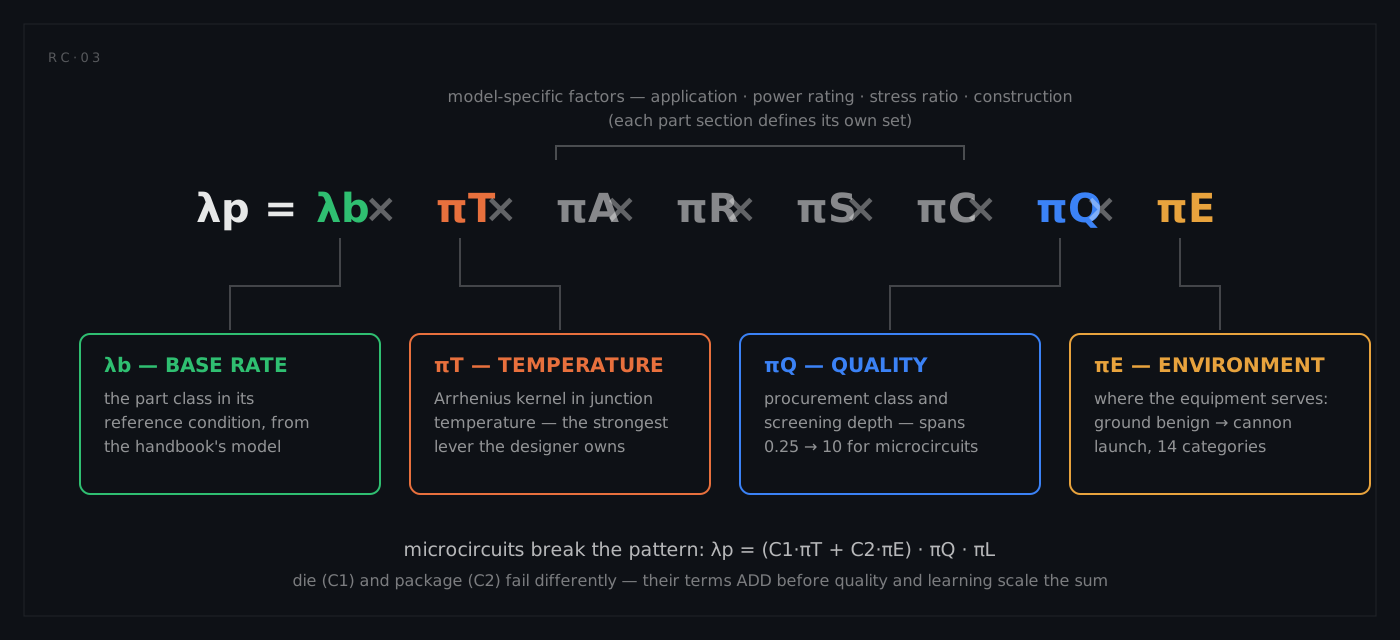
The part failure-rate model
Each part category in the handbook has its own model, but the family resemblance is strong. The typical form, the handbook's own example for discrete semiconductors, is:
λp = λb · πT · πA · πR · πS · πC · πQ · πE
where λb is the base failure rate of the part class in its reference condition and each π factor scales it for one influence: π_T temperature, π_A application, π_R power rating, π_S electrical stress ratio, π_C construction, π_Q quality, π_E environment. Quality and environment appear in nearly every model; the middle factors vary by part category, capacitor models bring capacitance and voltage-stress factors, resistor models bring power-stress factors, and so on.
Microcircuits are the notable exception, and the exception teaches the physics. Their model is additive at the core:
λp = (C₁·πT + C₂·πE) · πQ · πL
The die term (C₁, scaled by temperature) and the package term (C₂, scaled by environment) are separate because dies and packages fail differently: the die's failure mechanisms accelerate with junction temperature, while the package and its interconnects suffer from the vibration, humidity, and thermal cycling that the environment factor represents. Quality (π_Q) and learning (π_L: a penalty for devices in production less than two years) then scale the sum. In a benign environment the die term dominates; strap the same device to an airframe and the package term takes over.
Three further model shapes complete the family picture:
- K-factor notation. The UK and European handbook lineages write the same idea with different letters:
λp = λB · KE · KS, whereKSis a combined temperature-and-electrical-stress factor read from a two-dimensional table (stress ratio on one axis, temperature on the other). The notation differs; the physics and the workflow, base rate times environment times stress, are the same, and the tables carry the same lesson as π_T: the factor grid is normalised to 1 at a moderate reference condition and climbs steeply toward the hot, hard-driven corner. Cells beyond the sanctioned stress-and-temperature envelope simply don't exist in such tables, which is the tabular way of saying extrapolation is invalid. - Hybrids and multi-chip assemblies. A hybrid microcircuit is a small system pretending to be a part, and its model says so: the constituent dies contribute their own model rates (discounted, because a bare die escapes some of the packaged part's failure sites), and the substrate, its interconnections, and the package add their own terms, with quality and environment scaling the assembly. The teaching point survives any notation: for a hybrid, interconnect count and packaging density are reliability drivers in their own right, not packaging trivia.
- Additive cycling terms. Some parts carry a rate that is partly per-hour and partly per-event. The classic case is the connector: a mated pair accrues a base rate on the clock, plus a term proportional to how often it is mated and demated; at very low cycling frequencies the term vanishes, and on a test connector cycled daily it can dominate. Where a model shows an additive term, it is telling you a second failure mechanism with a second clock is present, worth knowing before you argue with the number.
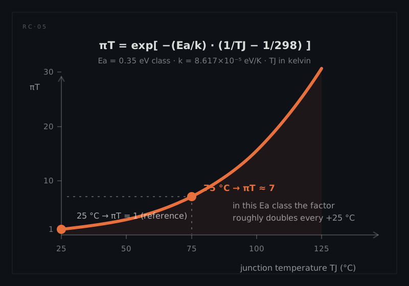
Temperature: the Arrhenius factor
The temperature factor deserves its own treatment because it is the strongest lever in the model and the one the design team can actually pull. Its kernel is the Arrhenius relationship: the same form chemistry uses for reaction-rate acceleration:
πT = exp[ −(Ea/k) · (1/TJ − 1/298) ]
with Ea the effective activation energy of the technology (electron-volts), k the Boltzmann constant (8.617×10⁻⁵ eV/K), and TJ the worst-case junction temperature in kelvin. At the 25 °C reference the factor is 1; above it, the rate climbs exponentially. Activation energies differ by technology: the handbook tabulates them per device family, so the steepness of the curve differs too; the microcircuit sections additionally carry a leading coefficient of 0.1 in their published π_T expression, one of several reasons to read each part section rather than assume one formula fits all.
The junction temperature itself is an input, not a guess. The handbook's procedure is explicit: get case temperatures from a thermal analysis of the equipment, then compute
TJ = TC + θJC · P
That is case temperature plus thermal resistance times dissipated power. If no thermal analysis exists yet, the handbook supplies default case temperatures per environment (45 °C for sheltered naval service, for example), defaults that are exactly what the part-stress pass exists to replace with real numbers.
The thermal resistance itself has a data hierarchy of its own. The manufacturer's datasheet θJC (junction-to-case) is the first choice; where airflow matters, the junction-to-ambient chain θJA = θJC + θCA extends it with the case-to-ambient leg, which depends on mounting and cooling. When a datasheet is silent, some standards, the European cycling-profile models among them, publish estimation formulas that reconstruct θ from the package family, its pin count, and an airflow factor, so the analysis never stalls for lack of a number. Every rung down this ladder adds uncertainty, and a good prediction report says which rung each hot part stood on.
Quality and environment
The quality factor π_Q encodes procurement class and screening depth, and its range surprises people seeing the method for the first time. For microcircuits the handbook's levels run from full space-grade screening to unscreened commercial parts:
| Microcircuit quality level | π_Q | Discrete semiconductor level | π_Q |
|---|---|---|---|
| Class S (space-grade screening) | 0.25 | JANTXV | 0.70 |
| Class B (full military screening) | 1.0 | JANTX | 1.0 |
| Class B-1 (MIL-STD-883 compliant) | 2.0 | JAN | 2.4 |
| Commercial / unknown screening | 10 | Lower quality | 5.5 |
| Plastic encapsulated | 8.0 |
A factor of 40 separates a space-grade microcircuit from an unscreened commercial one: in the model's eyes, procurement policy moves predicted reliability more than most design decisions. (The commercial-parts penalty is also the loudest single point of contention between the frozen 1995 models and modern component quality; more on that under pitfalls.)
The environment factor π_E places the equipment in one of fourteen service categories, from benign ground installations to gun-launched projectiles:
| Code | Environment | Typical service |
|---|---|---|
| GB | Ground, benign | air-conditioned equipment rooms, laboratories |
| GF | Ground, fixed | sheltered but unconditioned installations |
| GM | Ground, mobile | wheeled and tracked vehicles |
| NS | Naval, sheltered | below-deck, sheltered shipboard bays |
| NU | Naval, unsheltered | exposed topside shipboard equipment |
| AIC | Airborne, inhabited, cargo | transport-aircraft crew compartments |
| AIF | Airborne, inhabited, fighter | fighter cockpit environments |
| AUC | Airborne, uninhabited, cargo | transport equipment bays |
| AUF | Airborne, uninhabited, fighter | fighter equipment bays |
| ARW | Airborne, rotary wing | helicopters, internal and external |
| SF | Space, flight | orbital operation |
| MF | Missile, flight | free-flight missile phase |
| ML | Missile, launch | launch, boost, and re-entry loads |
| CL | Cannon, launch | gun-launched guided projectiles |
The spread is enormous: for microcircuits the environment factor runs from 0.5 in benign ground service to 220 for cannon launch. Choosing the environment category is therefore one of the highest-leverage decisions in the whole analysis, and one of the easiest to get subtly wrong when equipment spends its life in more than one of them.
Both factor families are model-specific, and that matters when programmes mix pedigrees. Quality scales don't translate: one handbook grades every part type on the same single quality ladder, another defines a different ladder per part class, so "quality level 2" means nothing without naming whose scale it is, and a practical criterion for choosing a model set is simply whose quality scheme matches how you actually buy parts. Environment lists don't translate either: the telecom-lineage models define only a handful of benign categories and have no naval or fighter environments at all, some model families use a much finer environment taxonomy than the fourteen above, and the mission-profile and cycling-profile models use no environment categories whatsoever, the profile itself carries the environmental story. The operational trap: ask a model for an environment it does not define and a naive tool returns a factor of zero, which silently zeroes the failure rate. A part with a suspiciously perfect predicted rate has usually fallen into exactly this hole.
Mechanical parts predict differently
Electronic prediction is a lookup discipline: the handbook regressed the field data, you supply the conditions. Mechanical prediction, the NSWC handbook's territory, is an engineering-calculation discipline: there is no tabulated base rate for "bearing"; the rate is computed from the design itself. Each mechanical component class gets a model whose base rate derives from design life, geometry, or material fatigue data, multiplied by a chain of modification factors, each driven by one physical parameter, actual-versus-rated load, lubricant viscosity at operating temperature, contamination level, surface finish, material hardness, misalignment. The flavour, per class:
| Component class | What drives its predicted rate |
|---|---|
| Bearings | Design B₁₀ life, load ratio, lubricant viscosity ratio, water contamination in the oil |
| Gears, splines | Applied torque vs rating, speed deviation, misalignment, lubricant, service-shock class |
| Springs | Material strength and modulus, wire and coil geometry, deflection per cycle, corrosion protection |
| Seals, gaskets | Contact pressure, hardness, surface finish, fluid pressure and viscosity, contaminant load, temperature vs material rating |
| Valves (poppet, spool) | Pressure differential, allowable leakage, seat geometry or spool clearance, fluid cleanliness |
| Actuators, cylinders | Wear physics: material pairing, side loads, stroke, contaminant hardness and concentration |
| Pumps and fluid drivers | Driver type (displacement types carry several times the base rate of centrifugals), flow and pressure ratios |
| Fasteners, shafts | Fatigue: endurance limit of the material, load type, size, surface treatment, thread manufacture |
Two structural differences from the electronic world deserve attention. First, many mechanical base rates are per cycle or per revolution, not per hour; the model converts through the operating tempo, which makes duty definition even more load-bearing than for electronics. Second, the inputs are real mechanical-design data: the method is usable exactly when the drawings exist, and data-hungry in proportion to its usefulness. The payoff for feeding it is a prediction that responds to design decisions, change a seal material, a filter rating, a spring deflection, and the number moves, which is precisely what a derating-style argument needs on the mechanical side of the BOM. In a mixed electro-mechanical roll-up, mechanical parts keep their own model under any electronic parent; the two families meet only at the summation.
Beyond the operating hour: dormancy, duty cycles, wear-out, and one-shot items
Everything so far has quietly assumed the equipment is switched on and the clock is running. Real missions are messier: hardware spends years on shelves, rides switched-off through transport, idles at partial duty, accumulates damage per cycle rather than per hour, wears out, or exists to work exactly once. A prediction that ignores these regimes isn't conservative, it is answering a different question than the one the mission asks.
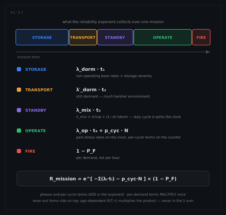
Dormant is not dead: storage and transport
A de-energised part still fails (seals dry, packages breathe, corrosion creeps, connectors fret in vibration), just far more slowly. Prediction handles this with non-operational rates: dormant failure rates typically sit an order of magnitude or more below operating rates, and the classic estimating shortcut (published in the Rome Laboratory reliability toolkit's dormancy topic) applies part-type-specific conversion factors to the active rates, a few percent of the active rate for connectors at one extreme, a few tens of percent for switches, relays and transformers at the other. Two structural points carry over from every model family that treats dormancy seriously. First, the dormant environment matters as much as the dormant state: sealed long-term storage in a controlled building is the gentlest condition there is, ordinary warehouse or shipboard stowage is harsher, and transport of switched-off equipment is a dormant environment too, usually the harshest one the equipment ever sleeps in, especially carried externally on a vehicle or aircraft. Second, dormant contributions are conventionally applied at equipment level with a single storage-environment factor rather than agonised over part by part; the precision lives in the active prediction, the dormancy correction is deliberately coarse.
Why bother? Because for long-storage systems (missiles in canisters, spares in depots, standby plants), the dormant λ·t term is the reliability question: twenty years of shelf at a tiny rate can outweigh minutes of flight at a large one.
Duty cycle: which clock is the MTBF on?
Handbook rates are per operating hour. Equipment energised 30% of the calendar accrues operating failures on 30% of the clock and dormant failures on the rest:
λcalendar = d · λoperating + (1 − d) · λdormant
with d the duty cycle. The consequences are larger than the formula looks. The same box owns two MTBFs, one against the operating-hour clock and one against the calendar, and both are correct; contracts, spares models, and field measurements routinely mix them up, because field MTBF is almost always measured on the calendar while predictions are quoted on the operating hour. A prediction report that does not say which clock its MTBF runs on has left its most litigated ambiguity unresolved. Phase-structured missions push the same logic further: each phase carries its own environment, temperature, duty cycle, and therefore its own phase rate, and the mission result is the time-weighted combination, exactly the multi-phase exponent from the foundations section.
Items that wear out
The constant-rate roll-up carries a silent assumption: anything that wears out gets replaced by preventive maintenance before wear-out failures matter. Where that policy actually holds, excluding wear-out from the prediction is correct. Where it is in doubt: no scheduled replacement, or service lives stretching toward the item's mean life, the wear-out-prone items must be pulled out of the λ sum and evaluated separately, because no constant rate can represent them.
The screen is cheap: flag any item whose required service time is no longer small against its estimated mean wear-out life; once the demand runs into a meaningful fraction of the mean, constant-rate treatment is over. The evaluation is conditional reliability. For an item of age T facing a further mission of duration τ:
R(T, τ) = R(T + τ) / R(T)
That is the probability of surviving the mission given survival to its start, and it degrades as T grows, which is the whole point: a wear-out item's mission reliability depends on the system's age, something the exponential can never express. Wear-out lives are usually modelled with a Weibull distribution of shape β > 1, or, where the failures cluster tightly about a mean life, with a normal distribution truncated at zero; before test data exists the scatter has to be assumed, and the assumption belongs in the report next to the result. The assumption matters directionally: the wider the scatter, the earlier wear-out failures start eroding reliability, a tight distribution keeps wear-out negligible until well past half the mean life, a loose one does not. The wear-out survival probabilities then multiply back into the system reliability alongside the constant-rate blocks, the mission product takes both, as the figure above shows. And the honest closing move: every item handled this way is a line in the maintenance plan, because the analysis just quantified what the preventive replacement interval is protecting.
One-shot devices
Igniters, release cartridges, thermal batteries, squibs: items that act once, are consumed by acting, and often cannot be tested without being used up. Time-based rates are meaningless here: a one-shot device carries a per-demand failure probability PF, its reliability is 1 − PF, and the evidence behind it comes from firing-trial populations, not operating hours. Method discipline follows: one-shot items are identified and kept out of the per-hour worksheets entirely, then multiplied into the system reliability at the demand point. Their boundary definition deserves contract-level care, a quoted demand probability may or may not include the firing chain's electronics, wiring, and connectors, and double-counting (or orphaning) that chain between the per-hour and per-demand halves of the model is a classic assembly error. Because required one-shot reliabilities are typically extreme and testing is destructive, the quantitative number leans harder than usual on process evidence, design margins, lot acceptance, environmental qualification, which is a large part of why one-shot reliability programmes feel more like quality engineering than statistics.