

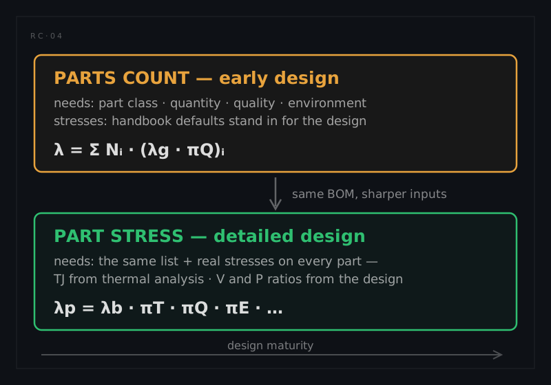
The handbook offers two procedures, and a real programme uses both, in sequence rather than in competition. Parts count is the early method: it needs only the generic part types, their quantities, quality levels, and the equipment environment, with handbook defaults standing in for every stress. Part stress is the mature method: it needs the real electrical and thermal stress on every part, and it is only possible once the design can supply them. Parts count usually errs conservative: its defaults are deliberately unflattering, so the walk from one to the other typically earns back margin.
Before the handbooks: the similar-equipment estimate
There is a rung below parts count, for the stage when even a rough parts list is fiction: estimate the new design's reliability from what comparable equipment actually achieved in service. Done honestly, it is a four-move analysis, not a guess. Define the proposed system: functions, performance, environments, timescale, and sketch its reliability model. Assemble comparators: similar equipment with known in-service reliability, ideally from the same design and manufacturing culture and similar environments, together with their development histories (how much growth testing, what problem areas, which failure modes dominated). Identify every significant difference between the comparator and the proposal, and adjust the comparator's reliability for each difference by an explicit, written engineering rule, for example, grading the novelty of each subsystem's technology on a declared scale and attaching a stated weighting to each grade. Then evaluate and report a best-case-to-worst-case range, not a single number, with the conditions behind each end stated, because the whole method rides on judgement-laden adjustments and deserves to look like it.
The similar-equipment estimate is systematically underrated. It is the only early method anchored to observed reliability rather than handbook regression; its weakness is transferability, which is exactly what the difference-adjustment discipline manages. Its output sets realistic targets and flags high-risk areas months before any parts-based method can run.
| Move | What it produces |
|---|---|
| Define the proposal | Functions, environments, timescale, and a reliability model |
| Assemble comparators | In-service reliability of similar equipment, with its history |
| Adjust for differences | A written engineering rule per difference: graded and weighted |
| Evaluate as a range | Best-to-worst case, with the conditions behind each end |
1. Choose the model set deliberately
The first decision is which models the programme will run, and it should be a contract-conscious one; mixed pedigrees in one roll-up need to be declared, because different handbooks embed different assumptions and units:
| Model set | Domain and character |
|---|---|
| MIL-HDBK-217F Notice 2 | Military electronics; parts count + part stress; frozen 1995; contractually entrenched |
| Telcordia SR-332 (Issue 4, 2016) | Telecom/commercial lineage (ex-Bellcore); FIT units; first-year multipliers; can blend lab and field data into the estimate |
| IEC 61709:2017 / SN 29500 | European industrial practice: Siemens' reference-condition rates converted to application conditions via IEC stress models |
| FIDES (2022 edition) | French aerospace/defence consortium guide; physics-of-failure-informed; mission-profile-driven, with an explicit process-quality audit factor |
| IEC TR 62380 | The European cycling-profile lineage (ex-RDF 2000): thermal and operating cycle counts drive the rate, and there is no environment table at all |
| 217Plus:2015 | Successor lineage to 217 (via RAC/RIAC); adds operating-profile and process-grade factors; supports Bayesian merge with own data |
| HRD5 (British Telecom) | UK telecom lineage; K-factor models with its own numbered environment scheme |
| GJB/Z 299B / 299C | Chinese military standard, structurally similar to the 217 family; 299C extends part coverage |
| NSWC-11 | Mechanical equipment; engineering equations from design and duty parameters, not tabulated part rates |
| NPRD / EPRD databooks | Field-observed rates for parts no parametric model covers; gap-filler, not a model |
Two companions are worth knowing whichever set you choose: ANSI/VITA 51.1 standardises input assumptions for 217F Notice 2 so that two analysts produce the same number from the same design, and IEEE 1413 is a framework for documenting a prediction, inputs, assumptions, data pedigree, uncertainties, so the number arrives with its provenance attached.
Model mixing has rules of its own. In practice a big roll-up is rarely single-pedigree (an electronics tree per one handbook, mechanical parts per the NSWC method, odd parts patched from field-data compendia), and that is legitimate as long as every deviation is declared and the units are reconciled. But the mission-profile and cycling-profile model families are a structural exception: their calculation basis (profiles instead of environment-plus-mission-time) is incompatible with mid-tree mixing, so they apply to the whole analysis or not at all. And any part the chosen model simply doesn't cover produces no rate, it needs an explicitly sourced rate or a different model, never a silent zero.
2. Frame the item and its mission
Define what is being predicted and where it serves. Select the environment category, and if the equipment sees more than one environment in use, segment the analysis: predict each mission phase in its own environment and time-weight the results by phase duration. The same goes for duty cycle: hours in the model are operating hours, and equipment that is energised 30% of the calendar needs that reflected, either in the profile or in how the result is quoted. This framing step is cheap, and errors in it are the expensive kind, they multiply everything downstream.
| Framing decision | Why it is load-bearing |
|---|---|
| Environment category | The largest single multiplier in the models |
| Mission phases | Each phase carries its own rates: the result is time-weighted |
| Duty cycle | Model hours are operating hours, not calendar hours |
| The MTBF clock | Decides how the result will meet the field data |
3. Build the part inventory
Pull the BOM into a part-class inventory: every line classified into a handbook category, with quantity, quality level, and, where the class needs it, complexity data such as gate counts, memory size, or package pin counts. This is data plumbing, and it is where a connected system model pays for itself: predictions built on hand-retyped BOM extracts inherit every transcription error and go stale at the first engineering change.
| Every part line carries | Example |
|---|---|
| Handbook category and subcategory | Fixed tantalum capacitor · 32-bit CMOS microprocessor |
| Quantity | 12 |
| Quality level, on that model's scale | Class B · JANTX · commercial |
| Complexity data where the class needs it | Gate count, memory bits, package pin count |
4. Run the parts count pass
The parts count equation is a single sum:
λEQUIP = Σ Nᵢ · (λg · πQ)ᵢ
That is quantity times generic rate times quality factor, summed over the part categories (microcircuits pick up the learning factor π_L as well; equipment spanning several environments computes per-environment and sums). The output is an early, defensible, usually conservative estimate, exactly what a proposal or an architecture trade needs.
5. Collect the real stresses
As the design matures, gather what the part-stress models need: worst-case junction temperatures from the thermal analysis (TJ = TC + θJC·P per part), applied-to-rated voltage and power ratios from the electrical design, application details per part category. Two handbook ground rules matter here: base rates may be interpolated between tabulated electrical stress values, but extrapolating beyond the tables, stress ratios above 1.0, temperatures beyond the tabulated range, is invalid. A part outside the tables is not a modelling problem; it is a derating finding that belongs in front of the design team.
| Stress input | Comes from |
|---|---|
Worst-case junction temperatures (TJ = TC + θJC·P) | The thermal analysis |
| Voltage and power stress ratios (applied ÷ rated) | The electrical design and derating worksheets |
| Application details per part category | Circuit design data |
| Duty and cycling counts | The operating profile |
Not every rate has to come out of a model. A specified rate (from the manufacturer, a databook, laboratory test, or the field) can replace the calculated one for any part, and often should: real evidence beats regression. Two disciplines keep this honest. Validate the outside number (under what environment, what confidence, what population was it measured?) and record its pedigree. And guard against double-counting field experience: if a part's specified rate already embeds field data, layering a field-data adjustment method or a correction factor on top of it applies the same evidence twice, silently. Every rate in the roll-up should be traceable to exactly one evidentiary basis.
6. Run the part stress pass and roll up
Compute λp per part from its category model, then roll up: sum the part rates per board, add the board-level contributions the handbook models separately (the printed wiring assembly, its solder connections, the connectors), and sum boards into units and units into the system. (Interconnecting wire between connectors is carried at zero rate; the connectors themselves are not.) The result is the system λ and MTBF, now traceable part by part.
| Roll-up line | Carried at |
|---|---|
| Every part | Its category model's λp |
| Printed wiring assembly | Its own handbook model |
| Solder connections | Per joint type |
| Connectors | Their own model, plus any cycling term |
| Interconnecting wire | Zero |
At system level the sum runs on effective rates, not always raw ones. A redundant group does not contribute the sum of its members; it contributes the (much smaller) effective rate the reliability model computes for the group, which for repairable redundancy depends on the repair time as well as the member rates. A subsystem that is present but not required for the mission contributes zero to the mission roll-up, even though it fails at its own rate and still costs maintenance, a scoping decision that belongs in writing on the reliability model, not in someone's head. One caution the algebra hides: a redundant group has no constant failure rate, its hazard is time-varying, so the reciprocal of its MTTF is not its failure rate, and treating it as one distorts any model downstream. This is precisely the seam where prediction hands over to the reliability block diagram, and the handbook says so: series arithmetic belongs to the prediction, redundancy structure to the modelling standard. Downstream of the roll-up the same rates are what the FMECA prices its criticality numbers with and what a quantitative fault tree uses for its basic events.
7. Document, compare, iterate
Record the assumptions (environment, temperatures, quality claims, data sources per part) with the result. Data provenance has a natural pecking order worth writing down: your own field data on similar products beats the manufacturer's data, which beats the handbook's generic tables; every part's rate should say which rung it came from, and contract-critical predictions typically need deviations from the agreed data source formally approved. Compare against the allocation. Then expect to do it all again: every design revision, every BOM change, every updated thermal analysis moves the number. A prediction is not a milestone deliverable that gets archived; it is a living estimate that tracks the design until field data retires it.