

Allocation's mathematics is short; its judgement content is not. This chapter covers both: the series arithmetic every method rides on, the weight-share-budget pipeline that all proportional methods share, the six-method family in detail, and the assumptions whose limits decide when an allocation is honest.
The budget arithmetic
Everything runs on one identity. Under the series assumption (any element failure fails the system), element failure rates add:
λgoal = Σ λᵢ
Failure rate is therefore the natural currency of allocation: rates divide like money, while MTBFs do not (two units of 40,000-hour MTBF make a 20,000-hour system, not an 80,000-hour one). The practical consequence: whatever form the top-level goal arrives in, the first move is to convert it into a failure-rate budget, split that, and convert back at the end for human consumption.
| Goal arrives as | Conversion to a rate budget |
|---|---|
| MTBF goal (hours) | λ* = 1/MTBF, in the project's declared unit (f/10⁶ h or FIT) |
| Reliability over a mission, R* at t | λ* = −ln(R*)/t under the constant-rate assumption |
| Availability goal Ai with known MTTR | λ* = (1/Ai − 1)/MTTR, valid where Ai is the steady-state inherent availability and MTTR is the whole downtime per failure; an operational-availability target has to be converted through mean downtime first |
| Failure-rate budget directly | Nothing: already the working currency |
The constant-rate machinery behind these conversions (the exponential distribution, its scope and its blind spots) is covered on the prediction foundations page and is not repeated here; allocation simply inherits it. What matters locally is discipline about units and clocks: an allocation quoted in FIT against a prediction quoted in failures per 10⁶ hours, or a mission-time R(t) target compared at the wrong t, produces margin arguments that are pure bookkeeping artefacts.
Every proportional method then follows the same three-step pipeline:
weight wᵢ per child → share = wᵢ / Σw → allocated λᵢ = share × λgoal
The methods differ only in where the weight comes from. One structural convention follows from the pipeline: a larger weight means a larger failure-rate allowance, a more lenient reliability target. Methods therefore weight upward the elements that are complex, immature or harshly placed, because those are the elements that cannot honestly promise rarity of failure. AGREE is the family's exception to the pipeline itself: it reaches the same conclusion through a closed form rather than a normalised share, and what it conserves is a weighted quantity rather than the raw rate, as the AGREE subsection sets out in full.
The method family
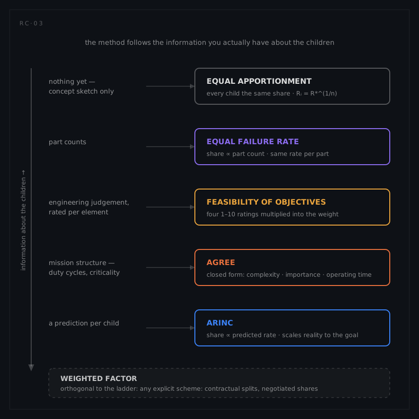
Choosing an allocation method is not a matter of taste; it is a statement about what you know. The six methods in common practice sit on a ladder of information, and a programme typically climbs it as design knowledge accumulates, often using different methods at different levels of the same tree in the same week.
| Method | Weight wᵢ | Information it needs | Character |
|---|---|---|---|
| Equal apportionment | 1 | None | Honest ignorance: a placeholder, not a position |
| Equal failure rate | part count nᵢ | Part counts | Complexity by proxy |
| Feasibility of objectives | product of four 1–10 ratings | Structured engineering judgement | The workhorse when data is thin |
| AGREE | closed form | Module counts, importance, operating times | Mission-aware; duty cycles and criticality |
| ARINC | predicted λᵢ | A prediction per child | Respects reality, scales it to the goal |
| Weighted factor | anything explicit | A declared scheme | Contractual and negotiated splits |
Equal apportionment
With n children and nothing known about them, each gets an equal share of the log-unreliability: Rᵢ = (R*)^(1/n), equivalently λᵢ = λ*/n. It is the only defensible split on day one and the least defensible split on any later day. Its whole value is that it is visibly provisional: a flag that the real allocation has not happened yet.
Equal failure rate per part
The first refinement money can't buy: weight each child by its part count, wᵢ = nᵢ, so every part in the system carries the same rate allowance. It encodes one true idea (more parts, more opportunities to fail) and nothing else: no technology, no stress, no environment. Useful exactly as long as part counts are the only real data on the table.
Feasibility of objectives
Developed in the US Army design-for-reliability handbook lineage primarily for mechanical-electrical systems without repair, and codified in MIL-HDBK-338B: each child is rated 1 to 10 on four factors by engineering judgement, independently scored and then reconciled in the open, entry by entry, when several engineers rate the same tree.
The rating sheet is the method, so it is worth seeing one. The anchors below are an example, written for a wayside signalling programme, and they are the ones the worked example scores against. Intermediate values interpolate: a 6 on environment is worse than a sheltered cabinet and better than trackside. Every programme writes its own sheet, in its own equipment's language, and archives it with the allocation.
| Factor | 1 | 5 | 8 | 10 |
|---|---|---|---|---|
| System intricacy | One board, few interfaces | A few boards and a backplane, one external protocol | Multi-board unit with its own power conversion and two protocol stacks | Interacting subsystems, several protocols, internal redundancy management |
| State of the art | Catalogue hardware with a decade of fleet history in this role | Current-generation variant of something the team has already fielded | First programme use of a technology the industry has fielded | Nothing comparable has been built; the design waits on laboratory work |
| Performance time | One short phase of the mission | About a quarter of the mission | Most of the mission, brief idle periods | Continuous, including standby between missions |
| Environment | Climate-controlled indoor rack | Sheltered outdoor cabinet, mild thermal cycling | Trackside or vehicle-mounted: temperature swings, vibration, condensation | Unprotected: salt, dust, shock, full ambient extremes |
The four ratings multiply into the weight, wᵢ = r₁·r₂·r₃·r₄ (spanning 1 to 10,000), shares normalise as usual, and λᵢ = shareᵢ × λ*. The multiplication is deliberate: an element that is complex and novel and always-on and exposed compounds its claim on the budget. The method's integrity lives entirely in the written ground rules behind the ratings, what exactly earns an 8 on state-of-the-art, because unanchored ratings are negotiable, and negotiable ratings get negotiated.
AGREE
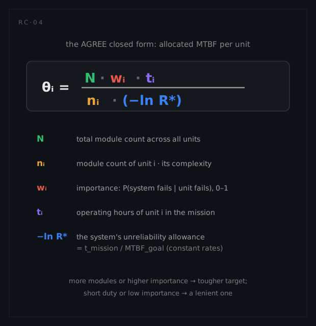
The 1957 AGREE report allocated a system reliability requirement over its units by three quantities: complexity (the unit's share nᵢ/N of the system's module count), importance wᵢ (the probability that the system actually fails when the unit fails, 1 for indispensable units, lower for degraded-mode survivable ones), and the unit's operating time tᵢ within the system's mission. The report's own expression works in reliability terms; in the small-unreliability regime it reduces to the closed form used in practice:
θᵢ = (N · wᵢ · tᵢ) / (nᵢ · (−ln R*))
with θᵢ the allocated unit MTBF and −ln R* = t / MTBFgoal the system's unreliability allowance over the mission. The intuition survives the algebra: each module in the system gets an equal slice of the system's allowed unreliability; a unit built from more modules therefore receives more of that allowance and a lower allocated MTBF, which is the more lenient target, while importance tightens it and a short duty loosens it. The topic's worked example shows the direction plainly: a five-module antenna carries 732,000 hours, a forty-module radio 91,500, eight times looser on eight times the modules. AGREE is the method of choice for electronics programmes where duty cycles and criticality genuinely differ between units, the two effects the simpler methods cannot see. Its guard rails: the underlying arithmetic is serial; treating redundant groups with it needs care the original report does not supply.
Importance is the input most often invented at the desk, and it does not have to be. wᵢ = P(system fails | unit fails) is a question two sibling analyses already answer for the same tree: the FMECA classifies every unit's failure effects at system level, which is that probability in words, and the RBD answers it structurally wherever a unit sits on a redundant path, where the loss of one member leaves the function standing. An importance figure that traces to one of those is defensible in review; one that appeared in a spreadsheet is a negotiating position.
What AGREE conserves is worth spelling out, because it is not what the rest of the family conserves. Invert the closed form and a unit's allocated failure rate is λᵢ = nᵢ · (−ln R*) / (N · wᵢ · tᵢ), with importance and operating time now in the denominator. A unit that is energised for part of the mission, or that the system can survive the loss of, is therefore handed a hardware rate several times larger than a share of the parent budget would have bought it, because only a fraction of that rate ever reaches the mission. The quantity that does sum to the parent is the discounted one, with t the mission time that both R* and the duty fractions are quoted against:
Σ λᵢ · wᵢ · (tᵢ / t) = (−ln R*) / t = λ*
AGREE conserves the duty-weighted, importance-weighted contribution to mission failure, not raw hardware rate, so wherever a unit runs for less than the full mission or the system can survive its loss, the level fails a naive rate-sum check by construction; only where every wᵢ is 1 and every tᵢ equals the mission time do the two currencies coincide and the raw sum close. In the worked example the gateway's three units carry 10.93 + 37.40 + 1.37 = 49.70 per 10⁶ h of hardware rate against a parent budget of 16.39, three times over on the naive check. Discount the fallback path by its importance and its duty fraction, 0.274 being its 200 hours in a 730-hour mission, and the level closes: 10.93 + 0.4 × 0.274 × 37.40 + 1.37 = 16.40. The conservation rule the results chapter states, children summing exactly to the parent level by level, holds at an AGREE level in that weighted currency and in no other. Reconcile an AGREE split there, and record the wᵢ and tᵢ next to the budgets, because a reviewer who rate-sums the rows will otherwise report an overrun that does not exist.
ARINC
The ARINC apportionment technique, from ARINC Research Corporation's early reliability engineering literature, weights each child by its present failure rate, observed or predicted: wᵢ = λᵢ,pred / Σλ,pred, so λᵢ,alloc = wᵢ · λ*. Its stated assumptions are the strictest of the family: series elements, constant failure rates, and child mission time equal to system mission time.
What ARINC really encodes is a policy: everyone improves by the same ratio. Every child's target is its predicted value scaled by the single factor λ* / Σλ,pred, so the relative standing of the children is preserved exactly. That is defensible when the prediction reflects genuinely comparable maturity across children, and quietly unfair when it doesn't: the element that already invested in reliability gets the same percentage squeeze as the one that hasn't. ARINC is honest about today; it has no opinion about potential, which is precisely the judgement the ratings methods exist to add.
Weighted factor
The escape hatch: one explicit weight per child, from any declared scheme: contractual splits between consortium partners, negotiated shares, imported results of an external optimisation. Its virtue is transparency; its risk is that "explicit" quietly degrades into "arbitrary" unless the scheme's rationale is written next to the weights.
Beyond the six: allocation as optimisation
The literature family the six practical methods belong to also contains genuine optimisation formulations. MIL-HDBK-338B documents a minimisation-of-effort algorithm that distributes improvement effort so the goal is reached for the least total effort, and the research literature extends this to cost-function and dynamic-programming allocations. They are worth knowing for what they teach: allocation is, at bottom, a resource-assignment problem, and worth respecting for what they demand: a credible effort-versus-reliability cost model per element, which most programmes at allocation time simply do not have.
The minimisation-of-effort logic is worth carrying even without the cost model, because its answer is counter-intuitive: effort is not spread evenly. Sort the children by the reliability they hold today, weakest first, and raise only the weakest k of them to a single common value R₀ chosen so the series product reaches the goal, leaving every child above that line untouched. The right k is the smallest one whose R₀ still lands at or below the reliability of the first child left alone. Three children at 0.90, 0.95 and 0.97 over the mission make a system of 0.829 against a 0.90 goal. Lifting only the weakest needs R₀ = 0.90 / (0.95 × 0.97) = 0.977, which is above the 0.95 sibling and therefore not the cheapest split. Lifting the weakest two to a common R₀ = √(0.90 / 0.97) = 0.963 does land under the untouched 0.97, and 0.963² × 0.97 = 0.900 closes the goal. The child that is already good is asked for nothing, which is the whole point and the exact opposite of what ARINC's uniform squeeze does.
In practice the ratings methods are the working compromise: they encode the same "harder things get bigger budgets" logic without pretending to know the cost curves.
Assumptions and their limits
| Assumption | Where it breaks | The guard |
|---|---|---|
| Series structure (rates add) | Redundant groups: members do not sum to the group | Budget the redundant group as one element; design its internals in the RBD |
| Constant failure rates | Wear-out-dominated elements, per-demand items | Budget in the quantity that fits (per-demand targets for one-shot items) |
| Independent elements | Shared services, common causes | Allocate the shared service its own budget line; it is an element too |
| Weights are honest | Ratings without ground rules, stale predictions | Written rating criteria; re-run when predictions refresh |
| A budget is a target, not a fact | Reading allocated columns as achieved reliability | The allocated-vs-predicted comparison, kept current |
Two of these deserve emphasis. The series-only limit is not a defect but a division of labour: allocation hands a redundant group one budget, and how the group meets it (duplication, standby, voting) is reliability modelling, solved in the RBD, not in the allocation. And the target-versus-fact distinction is the cultural one: an allocation table full of satisfied-looking MTBF numbers describes obligations, not achievements, and stays meaningful only as long as something real, a prediction, then test data, is regularly held up against it.