

A fault tree is a Boolean model of one specific failure, drawn downward from the failure to the things that cause it. Everything in this chapter follows from that sentence: the symbols exist to say what kind of thing each event is, the gates exist to say how causes combine, and the arithmetic is the arithmetic of the resulting Boolean expression.
The top event decides the whole analysis
The top event is a single, precisely stated failure condition, with its effect, its phase and its detection state written into the wording. Loss of attitude information is not a top event. Misleading attitude on both displays, unannunciated, on final approach is one, and it is a different tree from the same failure annunciated, and different again from total loss of attitude information in cloud.
Three boundaries have to be fixed before the first gate is drawn, and all three are conventions rather than discoveries:
| Boundary | The question | What happens if it drifts |
|---|---|---|
| Physical | Which items are inside the tree, and what is an external input | Two branches quantified against different assumptions |
| Resolution | How deep basic events go: box, board, or component | Cut sets that cannot be compared with each other |
| Initial state | Configuration, phase, what is already inoperative | A tree that answers a question nobody asked |
Fault, failure, and the immediate cause
The tree is built by asking one question at every node: what is the immediate, necessary and sufficient cause of this event? Not the root cause: the immediate cause. The root cause appears several levels down, as a consequence of asking the near question repeatedly, and skipping levels is the most common way trees end up wrong.
A failure is an item not doing what it should. A fault is broader: the item can be working exactly as designed and still produce a fault at system level, because it was commanded to do the wrong thing. That distinction is why fault trees find things an FMEA does not. The classic taxonomy at any node:
| Category | Meaning | Example |
|---|---|---|
| Primary fault | The item fails inside its specified envelope | A relay fails to close, in benign conditions |
| Secondary fault | The item is exposed to conditions beyond its specification | The same relay, after a supply transient |
| Command fault | The item works correctly, at the wrong time or on a wrong input | The relay opens because the logic told it to |
The event symbols
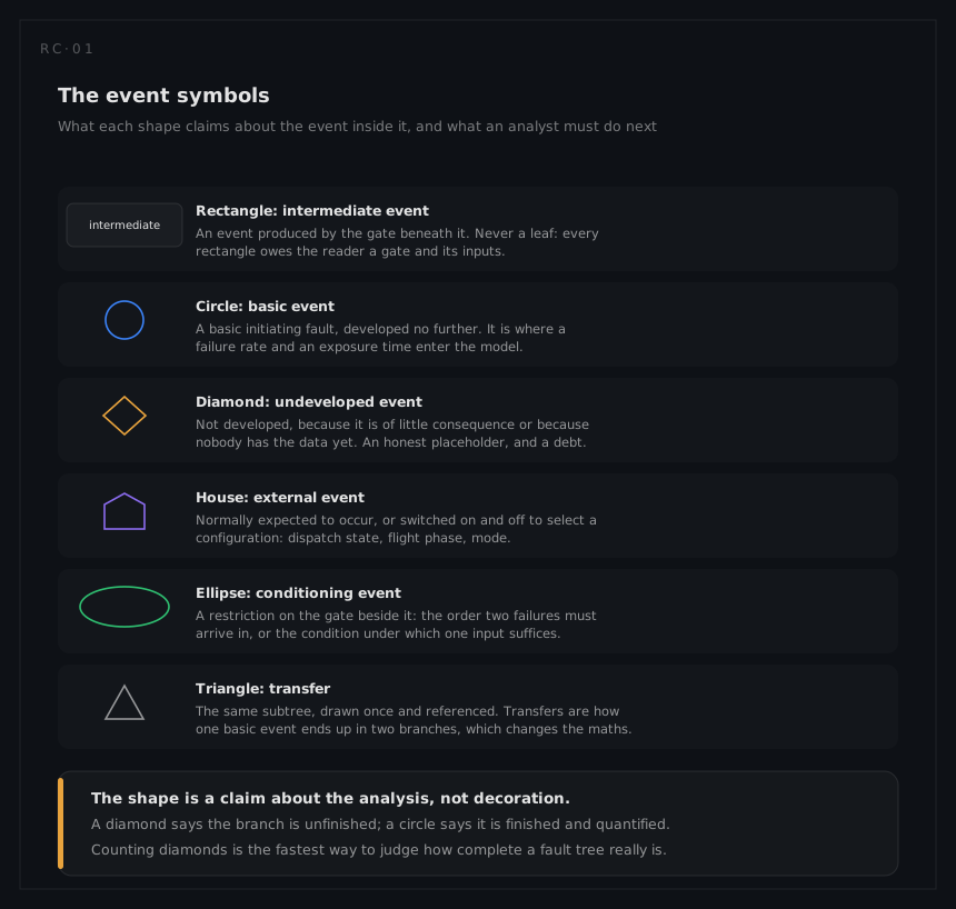
| Symbol | Name | What it asserts |
|---|---|---|
| Rectangle | Intermediate event | Produced by the gate below it; never a leaf |
| Circle | Basic event | A basic initiating fault, developed no further, carrying a rate and an exposure time |
| Diamond | Undeveloped event | Not developed, from low consequence or missing data |
| House | External event | Normally expected to occur, or switched to select a configuration |
| Ellipse | Conditioning event | A restriction on the gate beside it: an order, or a conditional probability |
| Triangle | Transfer | The same subtree, drawn once and referenced from elsewhere |
Two of those deserve emphasis. A house event is the cleanest way to model configurations: set it TRUE and the tree describes dispatch with an item inoperative, set it FALSE and it describes the normal fit, and one model answers both questions. And a transfer is where repeated events enter the model: the same basic event appearing under two branches is not two independent events, and any tool that treats it as such will quietly under-report the top event.
The gates
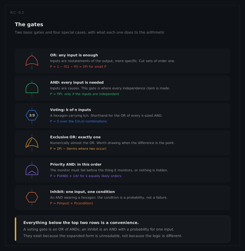
| Gate | Logic | The arithmetic | When it earns its place |
|---|---|---|---|
| OR | Any input | P = 1 − Π(1 − Pᵢ), and ≈ ΣPᵢ for small P | Inputs are restatements of the output, more specific |
| AND | Every input | P = ΠPᵢ, only if the inputs are independent | Inputs are causes, and redundancy is being claimed |
| Voting, k of n | Any k of the n | Sum over the C(n,k) combinations | Triplex sources, two-out-of-three logic |
| Exclusive OR | Exactly one | ΣPᵢ less the coincidence terms | When the coincidence is physically impossible and matters |
| Priority AND | All, in a stated order | P(AND) times an order factor, 1/k! for k equally likely orders | A monitor that must fail before the thing it monitors |
| Inhibit | One input, plus a condition | P(input) × P(condition) | The condition is a probability, not a failure: a phase, a crew response, a coincidence |
Every AND gate is a claim about independence, and it is the claim the whole quantification rests on. Two channels multiply only if nothing makes them fail together: not a shared power supply, not a shared cooling path, not a shared maintenance action, not a shared calibration constant, not the same design error in both. That is the entire reason the common cause analyses exist, and why a fault tree drawn without them is an optimistic document.
The inhibit and the conditioning event are where engineering judgement enters the model in numerical form, and they should be flagged as such wherever they appear. A conditional probability of 0.05 for the crew notices the discrepancy, or for two erroneous outputs agreeing closely enough to matter, is not measured; it is argued, and the argument belongs in the report next to the number.
Modelling the dependence an AND gate denies
Where independence cannot be fully shown, the answer is rarely to delete the AND gate. It is to keep the gate for the independent part and add a term beside it for the part that is not independent. Two models do that job, and both live in the tree as ordinary events.
The beta-factor model splits an item's failure rate in two: a fraction β is taken to fail every redundant channel at once, and the remaining 1 − β fails one channel on its own. In the tree that dependent fraction is a single basic event of probability β λ t, ORed in beside the redundant AND, so the branch becomes a sum of an independent product and a common term. The value of β is scored from the separation evidence rather than measured from failures, which is what makes it arguable.
The alpha-factor and multiple Greek letter models generalise the same idea past two channels, giving separate fractions for two-of-three and three-of-three coincidences instead of one lumped figure. They need more data than most programmes have, which is why the beta-factor form is what a fault tree usually carries.
The arithmetic is easy and the parameter is not. Applied to a redundant pair, any credible β will normally swamp the pair's independent product by orders of magnitude, and that is the real message: the credit a redundant architecture earns comes from the separation evidence, not from the multiplication. A tree that omits the term altogether has set β to zero without saying so.
Cut sets: the qualitative half
A cut set is a set of basic events whose joint occurrence causes the top event. A minimal cut set is one with nothing spare in it: remove any member and the top event no longer follows. Reducing the tree to its minimal cut sets is a Boolean operation, and it is the half of the analysis that survives when the data is doubtful.
The order of a cut set is the number of events in it, and order carries meaning that probability does not:
- Order 1 is a single point of failure. For a catastrophic condition it is prohibited outright, whatever the number attached to it.
- Order 2 is the working case for redundant designs, and every order-2 set is an independence claim that the common cause analysis has to support.
- Order 3 and above rarely matter numerically, and are where a common cause, if it exists, is usually hiding.
Cut sets also expose repeated events. If the same basic event appears in two branches, the naive product across an AND gate is wrong, because P(A · A) = P(A), not P(A)². Boolean reduction removes the error; multiplying gate by gate does not.
Quantification, and the approximations in it
Two families of numbers go on basic events, and mixing them is a common and expensive error:
unavailability, dimensionless for something already failed and waiting, and λ · t for something that fails during the exposure.
For a constant rate, the probability of failing within an exposure t is 1 − e^(−λt), and λt is the standard approximation, good to about 5 per cent while λt < 0.1. The top event is then computed either by the rare event approximation, summing the minimal cut set probabilities, or exactly by inclusion-exclusion. The sum is an upper bound and it is close whenever the individual sets are small, which in safety work they always are.
Both routes treat the basic event rates as exact, which they are not. Where the data is thin, the next step is a distribution on each rate, most often lognormal with a stated error factor, propagated to the top event by Monte Carlo so the answer is reported as a median with a 95th percentile rather than as a single figure. That is a different exercise from a sensitivity study on the assumptions, and it answers a different question: how much of the doubt comes from the data, and how much from the argument.
Exposure time is half the model
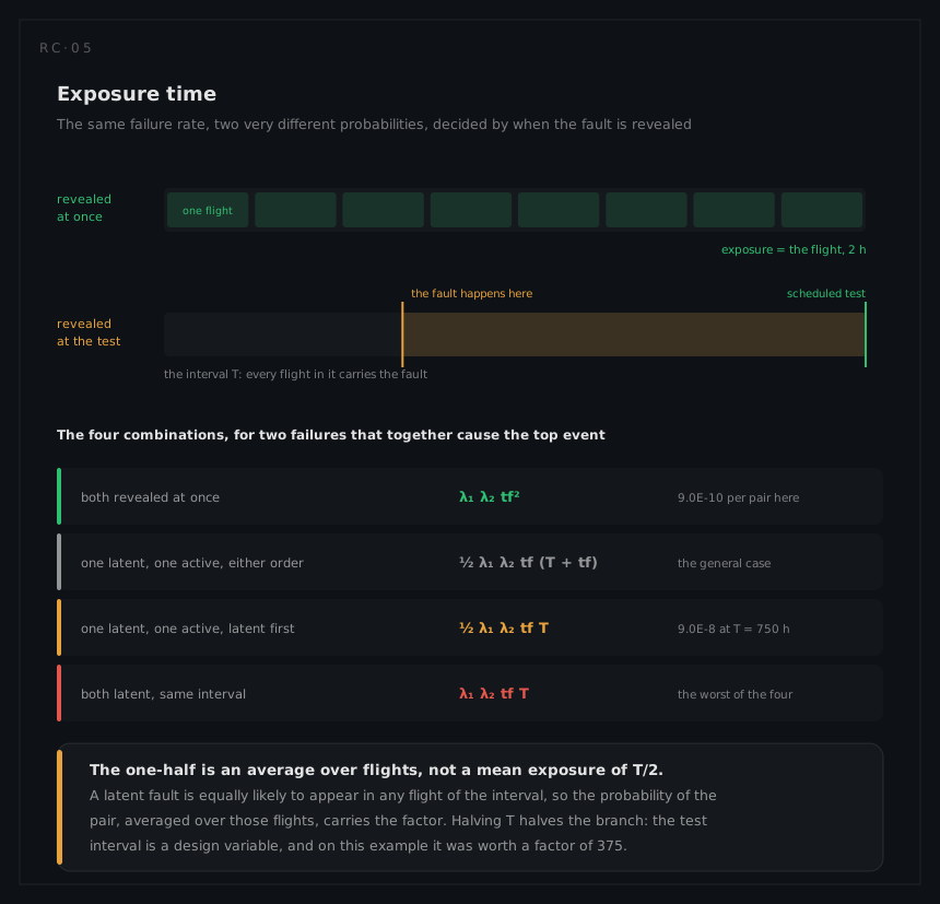
A fault revealed the moment it happens is exposed for the mission. A latent fault, revealed only at a scheduled test, is exposed for the interval between tests, which can be hundreds of times longer. Combining the two, for a pair of failures that together cause the top event, the standard forms are:
| Case | Probability per flight |
|---|---|
| Both revealed at once | λ₁ λ₂ tf² |
| One latent with interval T, one active, either order | ½ λ₁ λ₂ tf (T + tf) |
| One latent, one active, latent necessarily first | ½ λ₁ λ₂ tf T |
| Both latent, same interval T | λ₁ λ₂ tf T |
The one-half is worth understanding rather than memorising. A latent fault is equally likely to arise in any flight of the interval, so a pair's probability, averaged over the flights of that interval, picks up the factor. It is not a claim that the average exposure is T/2.
Two consequences follow. The test interval becomes a design variable, on the same footing as adding redundancy and usually far cheaper. And the analysis generates maintenance requirements: an interval assumed in a fault tree is a safety requirement, and if it later slips, the compliance argument goes with it.
What the tree cannot do
- It has no time in it. A static fault tree is a snapshot of one mission or one interval. Repair, reconfiguration, standby switching with imperfect coverage and sequence-dependent behaviour need a Markov model or a dynamic extension.
- It has no failure rate for design errors. Software and requirements errors can be drawn in the tree, and should be, but they carry no credible probability. Their purpose there is to show where the independence of two branches depends on the development process, which is what a development assurance level then governs.
- It only ever answers about the top event it was given. A tree is not a model of the system; it is a model of one way the system fails. A second failure condition means a second tree, and the two may share basic events and disagree about them if nobody checks.