

An evaluated diagram produces one primary number and several derived ones, and most of the trouble a block diagram causes downstream comes from the derived ones travelling without the primary. The rule that prevents all of it: a reliability result is a probability, a mission time and a success criterion, quoted together or not at all.
The primary result, stated properly
R = 0.978 over 720 hours, for "dry air above 6 bar at the actuator header", with all items serviceable at the start.
Every clause is load-bearing. Without the time the number means nothing; without the criterion it means something different to each reader; without the starting state it silently assumes a condition the plant may not be in. The worked example's 0.978 becomes a different number under a degraded-start policy, and the same diagram computes it.
| Reader | What they take from the result |
|---|---|
| The design authority | Whether the architecture meets the mission budget, and which change closes the gap |
| The allocation owner | The mission line of the budget, tested; the basic line is unaffected by any of this |
| Safety | A probability for a fault-tree gate, if and only if the criterion matches the top event |
| Operations | The availability result, if the blocks carry restoration times; the mission result on its own says nothing about downtime |
The two mean times, and why they disagree
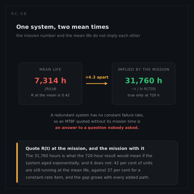
Two summaries are commonly asked for, and for a redundant structure they are far apart:
| Quantity | Worked example | What it actually is |
|---|---|---|
∫R(t)dt, the mean life | 7,314 h | The average time to the first system failure, dominated by behaviour long past any mission |
−t / ln R(t), the equivalent MTBF | 31,760 h at t = 720 | The constant rate a series item would need to match this result at this one time |
A factor of 4.3 between two legitimate answers, from one model. The tell that the system is not exponential is in the survival curve at its own mean: 42 per cent of systems are still running at 7,314 hours, against the 37 per cent an exponential item would show. Quote the equivalent MTBF into a contract and it will be read as a constant rate, which will then be used at a mission time it was never valid for.
Reading the cut sets
Cut sets rank a structure the way nothing else does, because they rank combinations rather than items.
- Order first. An order-1 cut is a single point of failure whatever its rate, and a design review's first question is how many there are and whether each is intended. The worked example has three, and they carry more than half its shortfall.
- Probability second. Within an order, the cut with the largest product dominates. In the worked example the largest order-2 cut is both compressors at 6.85 × 10⁻³, which is larger than any of the three order-1 cuts.
- Then look for shared elements. A cut set whose members share a supplier, a room, a power feed or a maintenance visit is not the order it appears to be. Two order-2 cuts sharing a cause are one order-1 cut wearing a disguise.
Summing cut sets as if they were disjoint (the rare-event approximation) overstates the answer, by 1.2 per cent in the worked example. For a system that mostly works the error is small and always conservative, which is why it is the standard practice for large models.
Importance: two rankings, two decisions
| Block | Birnbaum ∂R/∂Rᵢ | Its own q | Criticality |
|---|---|---|---|
| V · air receiver | 0.983 | 0.0057 | 25.2% |
| H · header | 0.981 | 0.0036 | 15.7% |
| F · intake filter | 0.980 | 0.0022 | 9.4% |
| C₁ · one compressor | 0.082 | 0.0828 | 30.3% |
| P₁ · one transmitter | 0.054 | 0.0284 | 6.8% |
| D₁ · one dryer | 0.043 | 0.0423 | 8.0% |
| X · cross-tie | 0.006 | 0.0178 | 0.5% |
The two columns rank the plant in almost opposite orders, and both are correct because they answer different questions.
Birnbaum importance is the sensitivity of system reliability to this block's reliability. It is a property of position, not of the block: the receiver's 0.983 says the system depends on it almost completely, and a percentage point of improvement there returns almost a full point at system level. This is the ranking that directs design effort.
Criticality importance multiplies that by how often the block actually fails, giving the probability that this unit is both failed and critical when the system goes down. The compressor tops it at 30.3 per cent despite the lowest-but-two Birnbaum score, because it fails far more often than anything else. This is the ranking that directs maintenance, spares and diagnosis effort. Note that criticality does not partition the shortfall: several units can be critical in the same failure, so the column is read row by row and not summed.
What to do with a result that misses
The comparison against the allocated mission budget has four honest dispositions, and one dishonest one.
| Finding | Response |
|---|---|
| A dominant order-1 cut | Add a path, or accept the single point explicitly and record why |
| A dominant order-2 cut with shared causes | Separate them: different supplier, different room, staggered maintenance. Usually cheaper than a third unit |
| Every cut small, the total still short | The block rates are the problem, not the structure; the shortfall flows back to the prediction and to design |
| Short by a margin smaller than the model's own uncertainty | Say so. Report the β sweep and the rate confidence rather than the point value |
| The number is short, so the diagram is redrawn | Not a disposition. If a criterion change is genuinely warranted, it is a change to the requirement and goes through the same review the requirement did |
What the result does not license
- It is not availability unless the blocks carry repair times. The mission result assumes nothing is restored. The same structure with an MTTR on every block gives availability, and it is a different number for a different question: 0.978 over the mission against 0.999877 at any moment.
- It is not a spares estimate. Spares are sized off the basic-reliability roll-up where every failure counts, which is the 521 per 10⁶ hours the diagram was built to argue with.
- It is not a constant rate. See the two mean times above.
- It is not more precise than β. The worked example's answer moves by a third of its shortfall between β = 0 and β = 0.1, and β is rarely known to better than a factor of two. Report the sweep with the result and the model stays honest about its own resolution.