

Everything an RBD computes follows from one object. Give each of the n blocks an indicator xᵢ that is 1 when the block works and 0 when it does not, and the diagram defines a structure function φ(x) that returns 1 when the system works. The function is coherent: repairing a block never breaks the system, and every block matters somewhere. Reliability is then the expectation of that function, R = E[φ(x)], and every formula below is a way of evaluating that expectation without enumerating 2ⁿ states.
Two standing assumptions come with it, and both are load-bearing. Blocks fail independently, so probabilities multiply. And each block is characterised by a probability of surviving the mission, Rᵢ = P(block i works throughout t), which for a constant-rate item is e^(−λᵢt) but need not be: a Weibull block, a demand-based probability of failure on demand, or a number from a test all sit in a diagram equally well.
The four structures that compose
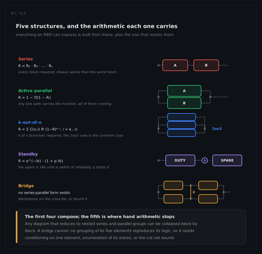
Series. Every block is required, so R = Π Rᵢ. Under constant rates this is the only structure in which failure rates add, λsys = Σ λᵢ, and it is the structure a parts-count prediction assumes for the whole system. A series chain is always worse than its worst block, and adding a block can only make it worse.
Active parallel. Any one path carries the function, all of them running: R = 1 − Π(1 − Rᵢ). For two identical blocks R = 2R₁ − R₁². The system's failure rate is not constant even when both blocks' rates are, which is the first place intuition breaks: a redundant pair ages, in the sense that the loss of the first unit changes the system's future, and no single λ describes it.
k-out-of-n. k of the n branches are required. For identical blocks:
Rkoon = Σ C(n,i) · Rⁱ · (1 − R)ⁿ⁻ⁱ for i = k … n
The 2-out-of-3 vote is the common case, R = 3R² − 2R³. Note where it sits: better than a single block while R > 0.5 and worse for every hour after that, the two curves crossing exactly at t = ln2 / λ. A voted group is a promise about a short mission, not about a long life, and quoting its MTTF hides that completely.
Standby. The spare is idle until a switch starts it. With a perfect switch and identical constant-rate units, the survival of the pair is the first two terms of a Poisson process:
R = e^(−λt) · (1 + λt)
and with a switch (or a detection, or a start) that succeeds with probability p:
R = e^(−λt) · (1 + p·λt)
The switch is the whole story. A cold spare with a perfect switch beats an active pair at every mission time; the same spare behind a 95 per cent start does not, and the worked example puts the break-even at p = 0.958. Warm standby sits between the two, the idle unit ageing at a reduced rate, and a diagram cannot represent it without leaving the boolean world.
What redundancy buys, and for how long
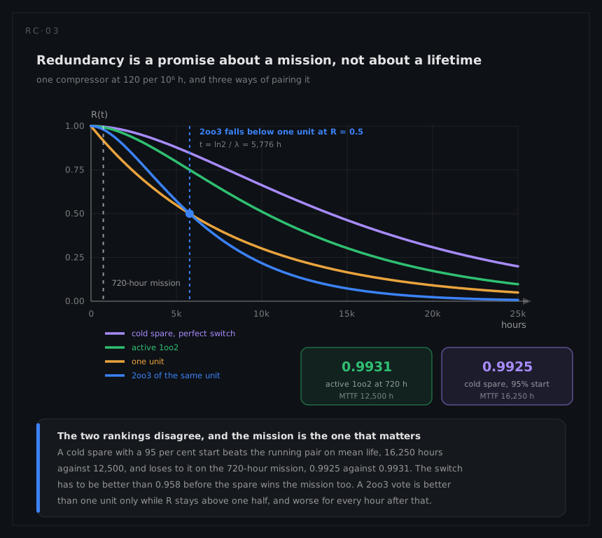
Mean time to failure is the integral of the survival curve, MTTF = ∫₀^∞ R(t) dt, and for the standard structures it has a closed form that is worth carrying in the head:
| Structure, identical units at rate λ | MTTF |
|---|---|
| One unit | 1/λ |
| Two in active parallel | 1.5/λ |
| Three in active parallel | 1.833/λ |
| Two in cold standby, perfect switch | 2/λ |
| Two in cold standby, switch probability p | (1 + p)/λ |
| 2-out-of-3 | 0.833/λ |
The last row is the one that surprises people: a 2oo3 vote has a shorter mean life than a single unit, because the second failure arrives long before the single unit's mean. It is nonetheless the right architecture for a short mission, where its reliability is much higher. Two measures, two rankings, and the mission is the one the contract cares about.
The structures that do not compose
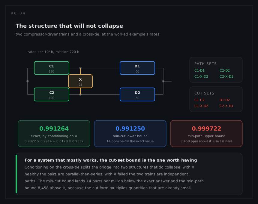
Collapsing a diagram block by block only works while the structure is nested series and parallel groups. The bridge is the smallest counterexample: two trains with a cross-tie between them, five elements, no grouping that reproduces the logic. Three routes out, in ascending order of effort:
Pivotal decomposition. Condition on one element and the rest collapses. Conditioning on the cross-tie X:
R = RX · R(structure with X working) + (1 − RX) · R(structure with X failed)
With X working the two compressors are parallel and the two dryers are parallel, in series with each other. With X failed the two trains are independent paths in parallel. At the worked example's rates that is 0.9822 × 0.9914 + 0.0178 × 0.9852 = 0.991264, which is exact.
Path sets and cut sets. A minimal path set is a smallest group whose survival is sufficient; a minimal cut set is a smallest group whose failure is sufficient. The bridge has four of each, and they are not the same four:
| Minimal path sets | Minimal cut sets |
|---|---|
| C₁·D₁, C₂·D₂ | C₁·C₂, D₁·D₂ |
| C₁·X·D₂, C₂·X·D₁ | C₁·X·D₂, C₂·X·D₁ |
Both descriptions determine the structure completely, and both over-count if their terms are simply multiplied, because the sets overlap. The correction is inclusion-exclusion, which is exact and grows factorially, or the Esary-Proschan bounds, which are one line each:
Π over cut sets (1 − Π qᵢ) ≤ R ≤ 1 − Π over path sets (1 − Π Rᵢ)
For a system that mostly works these two bounds are wildly asymmetric. The cut bound multiplies quantities that are already small and lands 14 parts per million below the exact answer; the path bound multiplies quantities close to one and lands 8,458 above it. The lower bound is the useful one, and it is the reason large fault trees and large diagrams are evaluated on their cut sets rather than their paths.
Enumeration. Five elements is 32 states, which a machine evaluates instantly and exactly. This is what a tool does, and the reason the hand methods still matter is that they say which combinations carry the answer, which enumeration does not.
Where independence fails
The independence assumption is the model's weakest joint, and it fails in three distinct ways that need three distinct treatments.
| What is shared | What it does to the diagram |
|---|---|
| A common cause: one event fails several blocks at once (a contaminated batch, a shared calibration error, a flood) | Split each block's rate into an independent part and a shared part; the shared part is a new block in series with the whole group |
| A support service: power, cooling, control air, an operator | It is a real block. Draw it once, in series with everything that depends on it, rather than assuming it away |
| Load sharing: the survivor works harder after the first failure | Not representable. The block rates are no longer constant across the mission, and the group needs a Markov model |
The first has a standard treatment, the β-factor: a fraction β of a block's rate is attributed to causes that take the whole redundant group, leaving (1 − β)λ independent. A pair with β = 0.1 is not a pair for a tenth of its failures, and since the shared term is in series with the group, no amount of further redundancy touches it. The method chapter works the sensitivity through; the short version is that β is usually the largest single uncertainty in a redundant model and is almost never measured.
Availability: the same structure, one more number per block
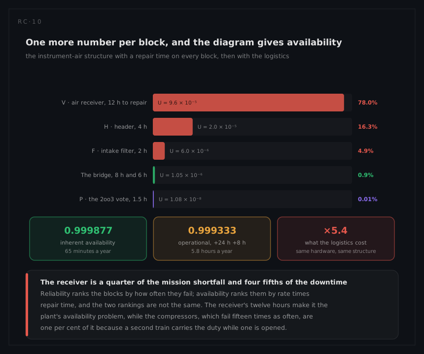
A block diagram becomes an availability model the moment each block carries a restoration time as well as a failure rate. The logic does not change at all. The structure function is the same function; only the quantity substituted into it moves from a survival probability to a steady-state availability.
For a block that fails at rate λ and is restored in a mean time MTTR:
A = MTBF / (MTBF + MTTR) = 1 / (1 + λ·MTTR), so U = 1 − A = λ·MTTR / (1 + λ·MTTR) ≈ λ·MTTR
and the structures compose exactly as they did for reliability: series multiplies availabilities, active parallel multiplies unavailabilities, k-out-of-n is the binomial on A, and cut sets multiply the unavailabilities of their members. A cut set of order two is now the probability that two blocks are down at the same moment, which is what makes redundancy worth so much more to availability than to reliability: the second compressor only has to outlast the eight hours its partner is being fixed, not the whole 720-hour mission.
Three conditions come with the steady-state form, and each has a name for what it excludes:
| The model assumes | What it excludes |
|---|---|
| Every failed block starts being restored immediately | One crew serving several blocks. Blocks then queue, and a queue couples them |
| Restoring one block does not change another's state | A repair that needs the system shut down, or a spare that two blocks draw from |
| The plant is observed in its steady state | The first mission, and any interval short enough that the transient still matters |
Operational availability is the same arithmetic with a longer clock on each block, because what keeps a plant down is rarely the repair itself:
MDT = MTTR + logistic delay + administrative delay, and Ao = MTBM / (MTBM + MDT)
The structure, the cut sets and the importance ranking are identical; only the number on each block changes. The worked example puts the two side by side, and the gap between them is a factor of five that no hardware change can touch.
The boundary is repair dependency, not repair. An RBD carries independent restoration perfectly well and is the standard tool for it. What it cannot carry is a shared crew, a queue for a spare, a repair that must wait for an outage, or a standby that ages at a different rate while it waits. Those are state problems, and they belong to a Markov model or to simulation.
What the model cannot say
A block diagram is a statement about one mission, evaluated at one instant, with blocks that do not come back. Four things follow, and they are limits of the technique rather than of any tool:
- No repair dependency. Independent restoration is fine, as above. A shared crew, a queue for a spare or a repair that waits for an outage is not: those couple the blocks, and the coupling is a state the structure function cannot hold.
- No sequence. "A fails then B" and "B fails then A" are the same state to a structure function. Where the order matters (a switch that must operate before the spare is loaded, a protection that must act before the damage) the logic is outside the boolean world.
- No phases, in one drawing. A mission with take-off, cruise and landing has three success criteria and therefore three diagrams, combined by multiplying the phase results for blocks that carry across.
- No modes. A block is up or down. A valve that fails open and a valve that fails shut sit on different paths, and only a FMECA can say which rate belongs in which block.