

Four outputs, and the programme usually reports the least useful one.
1. Where the design is now
| Report | The worked example |
|---|---|
| Instantaneous MTBF | 427 h at 5,000 test hours, as a point estimate |
| Cumulative MTBF | 278 h, alongside and never instead |
| β̂, and β̄ after the correction | 0.651, corrected to 0.615 |
| α, with its interval | 0.385, 0.08 to 0.58 |
| Failures, and the test type | 18, time-terminated at 5,000 h |
| Goodness of fit | C² = 0.014 against a 10 per cent critical value of 0.17 |
Instantaneous is the answer; cumulative is the arithmetic on the way there. The factor between them is 1⁄β̂, which is 1.54 on this test, and a report that gives only the lower number has understated the design by a third.
The interval belongs on α and on β, where the chi-square makes it exact. Putting those bounds through T⁄(nβ) to get a range on MTBF is tempting and wrong: it treats the observed failure count as the expected one, and the range it produces covers the truth about 75 per cent of the time while carrying a 90 per cent label. Quote the α interval, and quote the MTBF as a point estimate unless bound factors derived for MTBF itself are to hand.
Three of those rows are usually missing. The correction is exact and depends on the test type, so β̂ on its own is not a result. The interval on α is the difference between a finding and a picture: it clears zero here, so growth has been shown, and at this rate it would not have done so on fewer than about a dozen failures. And the goodness of fit is worth reporting with its own caveat, because at this sample size the test rejects a modest step change, 179 hours MTBF to 625, only a little over four times in ten.
2. Whether the requirement is reachable
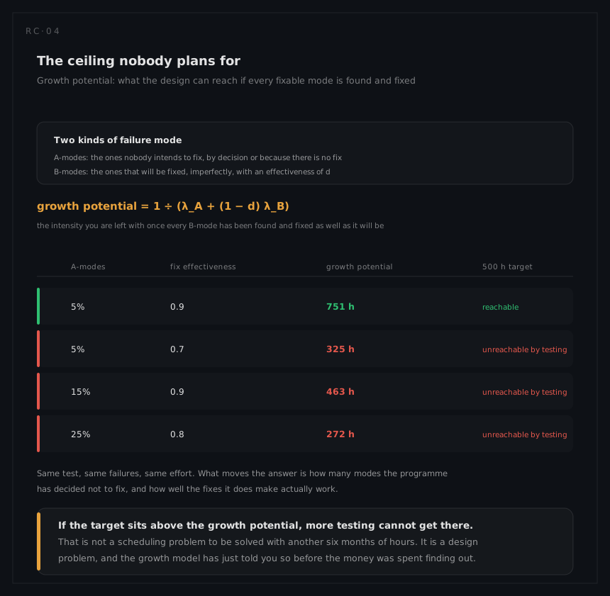
The growth potential, with the A-mode share and the fix effectiveness it was computed from, and a plain statement: reachable, or not reachable by testing. On the worked example the same test supports either answer depending on two judgements, which is exactly why both judgements belong in the report rather than in somebody's head.
3. What the schedule actually needs
Accumulated test time to the requirement, converted into calendar time at the programme's real test rate, with the corrective action periods included. On the worked example: 2,864 more test hours, which at twenty test hours a day and five days a week is six and a half more months, on top of eleven and a half already spent.
That number is the one that changes decisions, because it is usually larger than the schedule assumes and it arrives with enough arithmetic behind it to survive an argument.
4. The comparison with the field
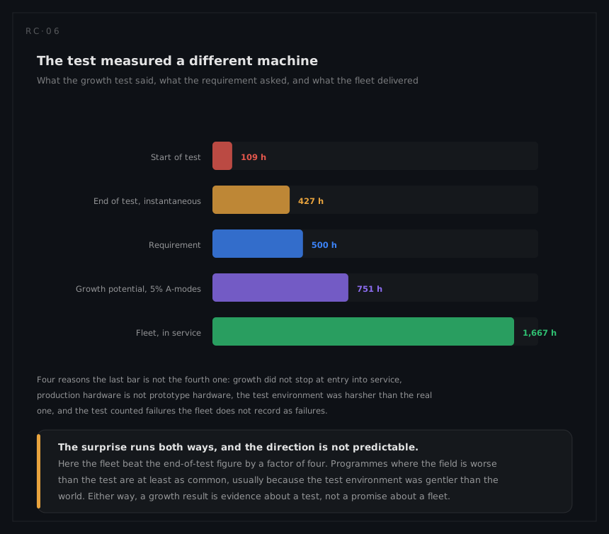
When service data exists, the observed rate beside the end-of-test figure, with the differences explained rather than averaged away. This is the only feedback the method receives, and an organisation that collects it for three programmes knows something about its own test environment that no handbook can supply.
What the results do not support
- A statement about field reliability. The test environment, the build standard and the counting rules all differ, and the direction of the error is not predictable.
- A demonstration of compliance. Growth improves a design; demonstrating a frozen one against a requirement with a stated confidence is a different test with a different plan.
- Extrapolation past the data. Projecting the curve out to meet the requirement on a chart is a plan, not a measurement, and the flattening makes the extrapolation optimistic.
- A conclusion from few failures. Two parameters from a handful of points give an interval wide enough to contain both success and failure; report it.
- Anything about modes the test never excited. What a test surfaces depends on what it stresses, which makes the environment part of the result and not part of the setup.