

Notation used in this topic
| Symbol | Reads as | Meaning |
|---|---|---|
N(t) | the number of failures counted by accumulated test time t | |
Λ(t) | big lambda of t | the expected number of failures by time t, E[N(t)] |
ρ(t) | rho of t | the failure intensity: the rate at which failures are arriving at time t, dΛ⁄dt |
| λ, β | lambda, beta | the two parameters of the power law process, Λ(t) = λ t^β; β below one is growth |
| β̂, β̄ | beta-hat, beta-bar | the maximum likelihood estimate of β, and the same estimate after its exact bias correction |
| α | alpha | the Duane growth rate, α = 1 − β |
| T, n | the accumulated time at which the test stops, and the number of failures in it | |
| tᵢ | the cumulative test time at the ith failure | |
m(t) | instantaneous MTBF, 1⁄ρ(t): what the configuration on test is worth at time t | |
t⁄N(t) | cumulative MTBF: total time over total failures, averaged across the whole test | |
χ²(p, k) | chi-square | the p quantile of a chi-square distribution on k degrees of freedom, which supplies the bounds on β |
C², M | C-squared | the Cramér-von Mises goodness-of-fit statistic, and the count it is computed on (M = n for a time-terminated test) |
| d, d̄ | fix effectiveness factor | the fraction of one mode's intensity that its corrective action actually removes, and the failure-weighted average across the modes being fixed |
λA, λB | lambda-A, lambda-B | the intensity of the modes nobody intends to fix, and of the modes that will be fixed |
h(T) | the rate at which previously unseen failure modes are still turning up at time T |
Every abbreviation used anywhere in RAMS Core is defined in the glossary.
The models are simple. What makes growth analysis hard is that the thing being measured keeps changing, which breaks the assumption every other reliability model rests on.
A process, not a distribution
Life data analysis fits a distribution to a population of identical items, each of which fails once. Growth analysis fits a process to a single item whose design is being modified while it runs, and which fails repeatedly. There is no population and no fixed distribution: there is a sequence of failure times, and an intensity that is expected to fall.
The mathematics is therefore a non-homogeneous Poisson process, a counting process whose rate changes with time. Write N(t) for the number of failures by time t, Λ(t) = E[N(t)] for its expectation, and the intensity ρ(t) = dΛ⁄dt for the instantaneous rate of arrival.
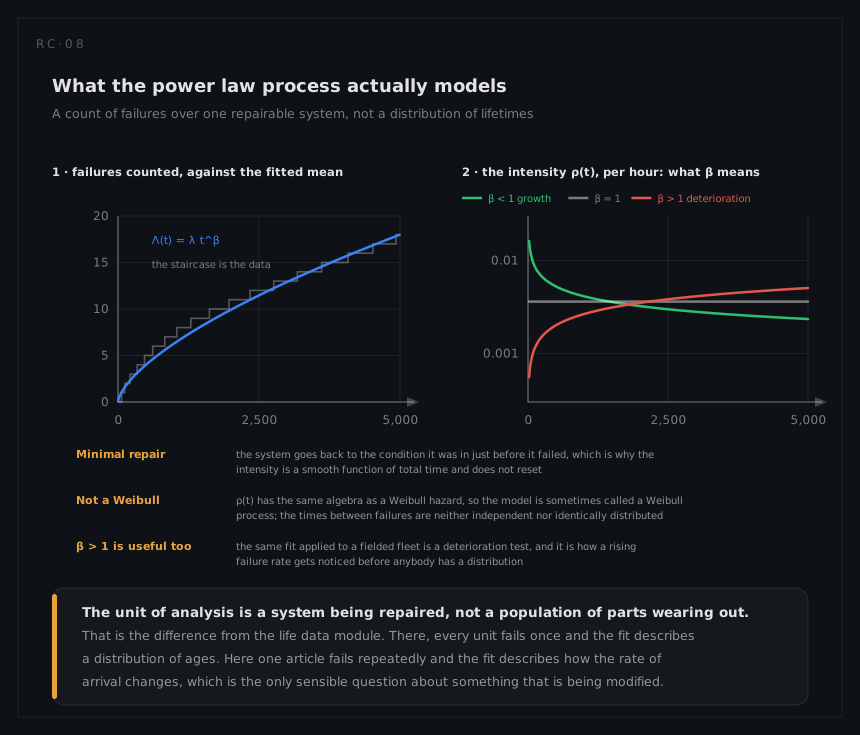
One assumption is doing quiet work here. The process is a minimal repair model: after each failure the system goes back to the condition it was in just before that failure, not to new. That is why the intensity is a smooth function of total accumulated time and does not reset at each repair, and it is a reasonable description of a complex system where one mode has been fixed and thousands of parts are untouched.
The Duane observation
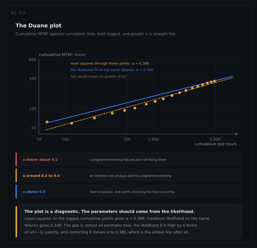
Duane's 1964 observation came first, and it was empirical: plot cumulative MTBF against cumulative test time on log-log axes during a programme with active corrective action, and the points fall near a straight line.
cumulative MTBF = t ⁄ N(t) ∝ t^α
where α is the growth rate, the slope of that line. Equivalently N(t) = K·t^(1−α), which is the whole model: a power law in the count.
The relationship everybody uses follows by differentiating rather than by assertion, and it is worth doing once because it is the source of the most common misreport in the field. If N(t) = K t^(1−α) then the cumulative MTBF is t⁄N(t) = t^α⁄K and the intensity is
ρ(t) = dN⁄dt = K(1−α) t^(−α)
so the instantaneous MTBF, 1⁄ρ(t), is t^α ⁄ (K(1−α)). Dividing one by the other, everything cancels except a constant:
instantaneous MTBF = cumulative MTBF ⁄ (1 − α)
The relationship holds only where the power law holds: it is exact inside the model and meaningless outside it.
| α | What it usually means |
|---|---|
| Below about 0.2 | Failures are being found and not effectively fixed |
| About 0.3 to 0.4 | An ordinary test-analyse-and-fix programme, working |
| Above 0.5 | Hard to sustain; check the failure scoring before celebrating |
Two cautions. α is an outcome, not a setting: it measures how well modes are being found and removed, and a programme that plans for a high α has planned to be lucky. And the Duane line is a graphical device with no statistics in it. Least squares will return a slope, but the points are not independent observations: the cumulative MTBF at the fifth failure contains all the data in the first four, so every point is correlated with every earlier one. The standard errors a regression package prints for that line are meaningless, and there is no goodness-of-fit test and no confidence interval to be had from it.
The power law process, or Crow-AMSAA

The same shape, stated as a statistical model, which is what the work at the US Army Materiel Systems Analysis Activity added. The expected number of failures by time t is
Λ(t) = λ t^β so the intensity is ρ(t) = λ β t^(β−1)
with β < 1 a falling intensity, which is growth; β = 1 a homogeneous Poisson process, which is no growth; and β > 1 deterioration. The bridge to Duane is direct: α = 1 − β.
It is not a Weibull distribution. ρ(t) has the same algebra as a Weibull hazard, which is why the model is sometimes called the Weibull process, and the name causes a specific and common error: treating the times between failures as independent draws from a Weibull. Under minimal repair they are neither independent nor identically distributed. The Weibull module fits ages at which units died; this fits the rate at which one system throws up failures.
Estimating it
For a time-terminated test, n failures at times tᵢ, stopped at T:
β̂ = n ⁄ Σ ln(T ⁄ tᵢ) and λ̂ = n ⁄ T^β̂
For a failure-terminated test, stopped at the nth failure, the sum is arithmetically the same, because ln(tₙ⁄tₙ) = 0 adds nothing. What differs is everything downstream: the bias correction and the bounds.
Two identities are worth keeping in the head, because they make most reporting checkable without a tool. At the end of test, cumulative MTBF is T⁄n by definition, and
instantaneous MTBF at T = T ⁄ (n β̂)
so the two differ by exactly 1⁄β̂, which is the same factor 1⁄(1−α) the Duane derivation produced.
The bias, which is exact
The maximum-likelihood β̂ is too big, and by a known amount rather than an estimated one. Conditional on n failures, the failure times are the order statistics of n draws with CDF (t⁄T)^β, which makes Σ ln(T⁄tᵢ) a gamma variable and β̂ = nβ ⁄ Gamma(n,1). The expectation of the reciprocal of a Gamma(n,1) is 1⁄(n−1), so
| Test type | E[β̂] | Unbiased estimator |
|---|---|---|
| Time-terminated | β·n⁄(n−1) | β̄ = ((n−1)⁄n)·β̂ |
| Failure-terminated | β·n⁄(n−2) | β̄ = ((n−2)⁄n)·β̂ |
Both are exact, not asymptotic. On eighteen failures the two corrections are 5.9 per cent and 12.5 per cent, from the same failure times, which is the practical reason the test type has to be recorded rather than assumed.
The bounds, which are also exact
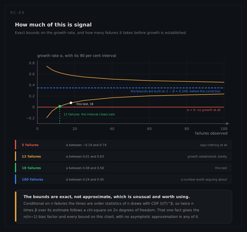
The same fact gives confidence bounds with no approximation in them. Since β̂ = nβ ⁄ Gamma(n,1) and twice a Gamma(n,1) is a chi-square on 2n degrees of freedom,
2nβ ⁄ β̂ ~ χ²(2n) for a time-terminated test, and χ²(2n−2) for a failure-terminated one
so a two-sided interval on β is β̂·χ²(a, 2n)⁄2n to β̂·χ²(1−a, 2n)⁄2n. This is worth using, because the interval is much wider than programmes expect. On a test with eighteen failures and β̂ = 0.65, the 90 per cent interval on the growth rate runs from 0.08 to 0.58.
The chart above turns that into the question a design review should ask: how many failures before growth is established at all? At this growth rate, twelve. Below about a dozen the interval still contains α = 0, and a growth curve presented on eight failures is a picture rather than a finding.
Does the model fit
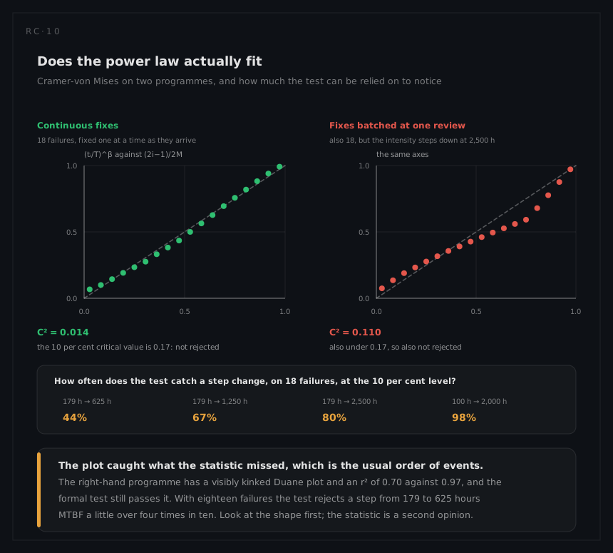
Goodness of fit for a time-terminated test is normally the Cramér-von Mises statistic, which compares the transformed failure times against the uniform they should be:
C² = 1⁄(12M) + Σ [ (tᵢ⁄T)^β̄ − (2i−1)⁄(2M) ]²
computed with the unbiased β̄ and M = n. Large means reject. Critical values depend only on M and are tabulated in the handbooks; for eighteen failures the 10 per cent value is about 0.17.
Its weakness is worth knowing before it is relied on. With eighteen failures, tested at that 10 per cent value, the statistic rejects a step change from 179 hours MTBF to 625 only a little over four times in ten. A programme that batched its fixes into one design review will very often pass this test while its Duane plot is visibly kinked. Read the shape first; the statistic is a second opinion, not a verdict.
The model's assumptions, which are routinely violated
- One system, or a pooled set of identical ones. Different build standards are different processes.
- Corrective actions applied as the test proceeds. Batch the fixes and the intensity is a step, which no power law can represent.
- No configuration change large enough to make the intensity discontinuous. A significant redesign mid-test starts a new process.
- A consistent definition of a chargeable failure, from the first hour to the last.
Which estimator for which data
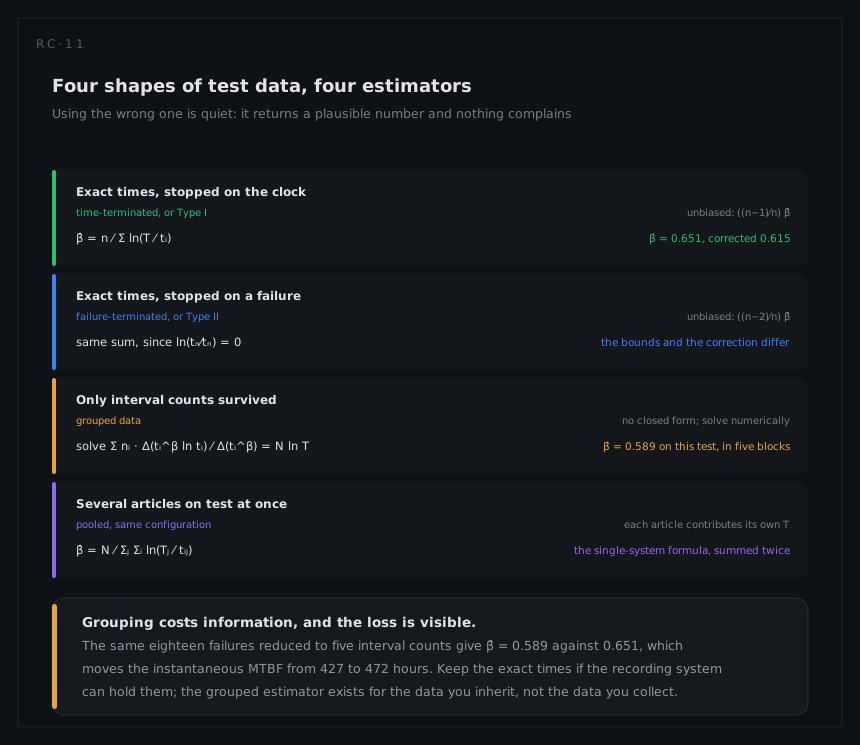
| The data you have | What to use |
|---|---|
| Exact times, stopped on the clock | β̂ = n ⁄ Σ ln(T⁄tᵢ), unbiased by (n−1)⁄n |
| Exact times, stopped on a failure | The same sum, unbiased by (n−2)⁄n, and bounds on 2n−2 degrees of freedom |
| Only interval counts | The grouped estimator, solved numerically: no closed form |
| Several articles at once | The same formula with the sums running over every article and its own end time |
Grouping costs information and the loss is measurable. The eighteen failures in the worked example, reduced to five interval counts, give β̂ = 0.589 against 0.651 from the exact times, which moves the reported instantaneous MTBF from 427 hours to 472. The grouped estimator exists for the data you inherit, not the data you collect.
Planning, tracking, projection

| Activity | When | What it produces |
|---|---|---|
| Planning | Before the test | An idealised curve from the initial MTBF to the requirement, and the test time and management strategy needed to be plausible |
| Tracking | During the test | The model fitted to the failures so far, saying where the design is now |
| Projection | After a corrective action period | Where the design will be once identified fixes are embodied, using their expected effectiveness |
Conflating them flatters the programme, and the usual conflation is a planning curve shown at a review as though it were data.
Projection is the only one of the three that predicts, and it is built from three pieces rather than from the tracking fit: the intensity of the modes nobody will fix, the residual intensity of the fixed modes after allowing for how well the fixes work, and an allowance for the modes not yet seen, estimated from the rate at which new modes have been turning up. That third term is what separates a projection from an arithmetic recalculation, and it is also the one carrying most of the uncertainty.
A-modes, B-modes and the ceiling
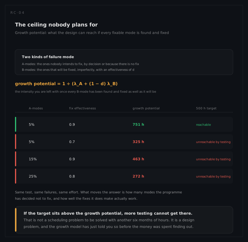
Every failure mode is classified before or during the test:
| Class | Meaning |
|---|---|
| A-mode | Will not be fixed, by decision, by cost, or because no practical fix exists |
| B-mode | Will be fixed, imperfectly |
The imperfection has a name and a number: the fix effectiveness factor d, the fraction of a mode's intensity that a corrective action actually removes. It is well below one in practice, and pretending otherwise is how growth plans become fiction.
The two together set the ceiling:
growth potential = 1 ⁄ (λA + (1 − d) λB)
If the requirement sits above the growth potential, no amount of testing reaches it. That is a design finding, and the arithmetic that produces it needs nothing more than the early failure data and two honest judgements.
What growth cannot tell you
- Nothing about the fleet. The environment, the build standard, the duty cycle and the failure-counting rules all differ between a test cell and service.
- Nothing about modes that never appeared. A test surfaces what the test environment excites, which is why the environment is part of the result.
- Nothing about a design that stopped changing. Once the configuration is frozen, the process model no longer applies and the right analysis is a distribution fitted to the failures, or a demonstration test.
- Nothing reliable from a handful of failures. Two parameters from six failures is an estimate with an interval wide enough to contain both success and failure, and now there is a chart above that says exactly how wide.