

Nearly everything else in this knowledgebase runs on a constant failure rate. A prediction produces one, an RBD multiplies them, a fault tree puts them on basic events, a repair level analysis turns one into an annual demand. The assumption is everywhere and it is almost always made without evidence, because at design time there is none.
Life data analysis is where the evidence arrives. It takes the ages at which units failed, and the ages at which units did not, and fits a distribution that says how the chance of failing changes with age. What comes out is one number that matters more than the rest: whether the hazard rises, falls or stays flat.
Why one parameter decides so much
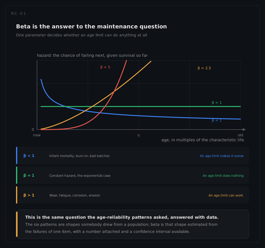
β | The item | What an age limit does |
|---|---|---|
< 1 | Gets more reliable with age: infant mortality, burn-in, bad batches | Makes it worse, by replacing run-in units with new ones |
= 1 | Constant hazard, the exponential case | Nothing at all |
> 1 | Wears out: fatigue, erosion, corrosion, contamination | Can work, and the fit says at what age |
That is the same question the age-reliability patterns ask, answered with the item's own data rather than with a population study from another industry. Where RCM asks whether a scheduled restoration or discard is applicable, this analysis is what answers it.
It is also the question a rate cannot answer. Two populations can produce the same ten failures in the same thousand hours, the same MTBF of 100 hours, and opposite maintenance policies: one where a tenth is dead inside two hours and scheduled replacement makes things worse, and one where nothing fails before fifty hours and a life limit is the obvious move. The worked example runs both of them from the raw failure times to the two decisions.
Where it sits
| Stage | What the analysis is for |
|---|---|
| Development test | Fitting life to test failures, usually with too few points to be confident |
| Early service | The first real distribution, and the first check on the constant rate everybody assumed |
| Mature service | Refits as the fleet ages, which is when the tail of the distribution finally has data in it |
| Warranty and support contracts | Expected returns over a period, which is a distribution question rather than a rate question |
| Fleet retirement | What the last years of life will cost, once most of the population is past its characteristic life |
What it is not
- It is not prediction. A prediction estimates a rate for hardware that has never run. This estimates a distribution from hardware that has.
- It is not a rate. The output is a function of age. Collapsing it into one number is legitimate only alongside the age or the fleet profile it was collapsed at.
- It is not automatic. Data has to be assembled per failure mode, with the age each unit reached, including the units that did not fail. Most of the work is in that sentence.
- It is not only Weibull. The Weibull is flexible enough to cover most hardware wear behaviour, but a lognormal fits repair times better and a mixture fits two competing modes better, and the plot is what tells you which.
Where the discipline comes from
IEC 61649 is the international standard for Weibull analysis, covering estimation, goodness of fit and confidence intervals. The wider dependability series carries the surrounding statistics: test conditions and principles, life testing, and the treatment of censored data. On the US side the reliability handbooks carry the same methods in an engineering register, and the freely available NIST Engineering Statistics Handbook is the reference most practitioners actually reach for. In the practitioner literature, Abernethy's handbook is the standard text and the source of much of the vocabulary, including the B-life notation this module uses.