

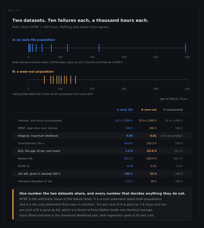
Two examples. The first is a clean comparison that shows what a life data analysis is for: two datasets that produce exactly the same MTBF and nothing else the same. The second is field data with survivors in it, which is what the analysis actually looks like in service. Every value on this page is an illustrative teaching figure.
Part one: two datasets, one MTBF
Two candidate designs for the same item are run to failure on the same rig, under the same duty cycle. Ten units of each. Both designs accumulate 1,000 hours across ten units and produce ten failures, so both acceptance reports carry the same headline:
MTBF = total time ⁄ failures = 1,000 ⁄ 10 = 100 hours
Both are complete samples with no suspensions, which is rare outside a test house and is the reason to start here: the arithmetic is visible all the way through. Ages at failure, in hours:
| Design | Failure times, hours |
|---|---|
| A | 1, 2, 6, 13, 24, 43, 72, 123, 222, 494 |
| B | 50, 70, 78, 89, 96, 103, 113, 120, 133, 148 |
Read the two rows before reading anything else. Design A lost three units inside the first six hours and had one unit still running at 494. Design B lost nothing at all before 50 hours and then lost everything within a hundred hours of that. Both average 100.
Plotting positions, which are the same for both
The plotting position depends on the rank and the sample size, not on the times, so this column is identical for the two designs and only the ages move. Bernard's approximation with N = 10:
i | F(i) = (i − 0.3) ⁄ 10.4 | A: t | x = ln t | y = ln(−ln(1−F)) | B: t | x = ln t |
|---|---|---|---|---|---|---|
| 1 | 0.0673 | 1 | 0.000 | −2.664 | 50 | 3.912 |
| 2 | 0.1635 | 2 | 0.693 | −1.723 | 70 | 4.248 |
| 3 | 0.2596 | 6 | 1.792 | −1.202 | 78 | 4.357 |
| 4 | 0.3558 | 13 | 2.565 | −0.822 | 89 | 4.489 |
| 5 | 0.4519 | 24 | 3.178 | −0.509 | 96 | 4.564 |
| 6 | 0.5481 | 43 | 3.761 | −0.230 | 103 | 4.635 |
| 7 | 0.6442 | 72 | 4.277 | 0.033 | 113 | 4.727 |
| 8 | 0.7404 | 123 | 4.812 | 0.299 | 120 | 4.787 |
| 9 | 0.8365 | 222 | 5.403 | 0.594 | 133 | 4.890 |
| 10 | 0.9327 | 494 | 6.203 | 0.993 | 148 | 4.997 |
The y column is shared too. Everything that separates the two designs is in the spread of x: design A's log-ages run across 6.2 units of the axis and design B's across 1.1, and since the slope of y against x is β, that ratio is the difference in β.
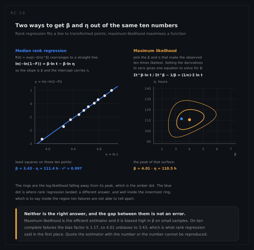
The fits
Least squares of y on x on those points, and then maximum likelihood on the same ten numbers:
| Design A | Design B | |
|---|---|---|
Rank regression β | 0.55 | 3.43 |
Rank regression η | 68.4 h | 111.4 h |
r² | 0.981 | 0.997 |
Maximum likelihood β | 0.60 | 4.01 |
Maximum likelihood η | 66.8 h | 110.5 h |
MLE β, bias corrected | 0.51 | 3.43 |
90 per cent interval on β | 0.33 to 0.81 | 2.20 to 5.42 |
The last two rows are the maximum-likelihood β worked on: divide it by 1.17 for the bias correction, and by 1.82 and by 0.74 for the two ends of the interval.
Three things in that table are worth stopping on.
The maximum-likelihood β is high in both cases, by about the same factor. That is the small-sample bias, not a property of either design: on ten complete failures the mean of β̂ ⁄ β is about 1.17. Divide by it and design B's 4.01 becomes 3.43, which is exactly what rank regression said without needing the correction. The two methods were never really in disagreement; one of them was reporting a known bias.
Neither interval contains 1. This matters more than the point estimates. Ten failures is not much data, and the obvious objection to the whole comparison is that the difference in shape could be chance. It could not: A's interval tops out at 0.81 and B's starts at 2.20, so the constant-hazard model is outside both of them. The two designs really do fail by different mechanisms, and the test was long enough to prove it.
The intervals are still wide. A factor of two and a half, in both. That is enough to settle the question being asked here, which is whether the hazard rises or falls. It would not be enough to settle a question that turned on β being 3.4 rather than 4.5.
The same fit, seen four ways
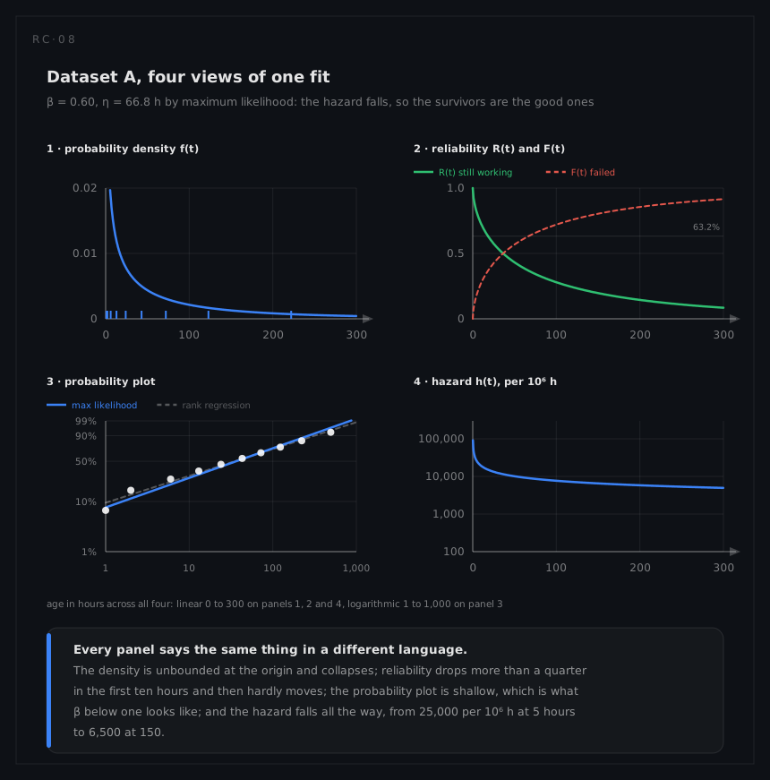
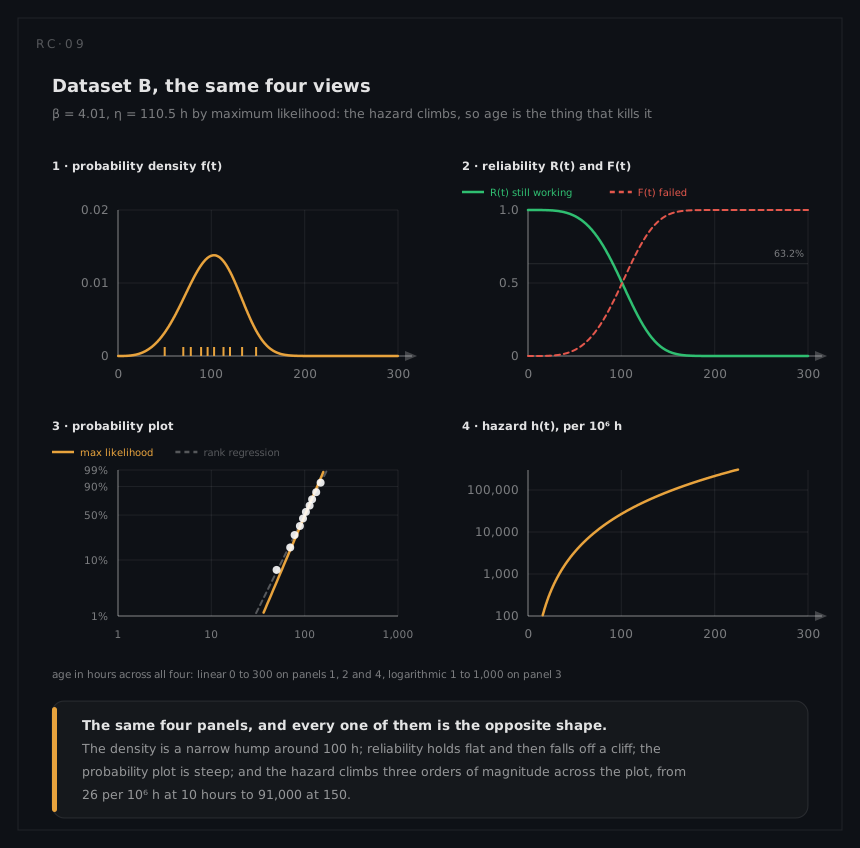
Nothing in those eight panels is a different analysis. They are the same two parameters drawn four ways each, and the reason to look at all four is that different decisions read different panels: procurement reads the density, a warranty reads the CDF, an analyst checking the model reads the probability plot, and maintenance reads the hazard.
Reliability, and the hazard underneath it
R(t), the fraction still working, against what the exponential with MTBF 100 h would have predicted:
| Age | A | B | If exponential |
|---|---|---|---|
| 10 h | 0.727 | 0.9999 | 0.905 |
| 25 h | 0.575 | 0.997 | 0.779 |
| 50 h | 0.432 | 0.959 | 0.607 |
| 100 h | 0.279 | 0.512 | 0.368 |
| 150 h | 0.197 | 0.033 | 0.223 |
The exponential is wrong about both, and not by a fixed factor or in a fixed direction. At 10 hours it is optimistic about A by a factor of three in failures and pessimistic about B by a factor of a thousand. By 150 hours the sign has flipped for B: the exponential has 22 per cent of them still working when 3 per cent are. It has not flipped for A, which the exponential over-predicts all the way out to 184 hours, so between about 114 and 184 hours the one model is optimistic about both designs at once. There is no age at which it is right about either.
And the hazard, h(t) = (β⁄η)(t⁄η)^(β−1), in failures per million hours:
| Age | A | B | Ratio A : B |
|---|---|---|---|
| 5 h | 25,286 | 3 | 7,700 |
| 10 h | 19,189 | 26 | 725 |
| 25 h | 13,324 | 416 | 32 |
| 50 h | 10,111 | 3,341 | 3.0 |
| 69 h | 8,895 | 8,798 | 1.01 |
| 100 h | 7,673 | 26,842 | 0.29 |
| 150 h | 6,529 | 90,816 | 0.07 |
The two hazards cross just past 69 hours. Before that A is the worse design by any margin you like; after it, B is. There is no answer to which design is more reliable that does not name an age, and the MTBF that both suppliers quoted is the one number that cannot name one.
The question a maintenance programme actually asks
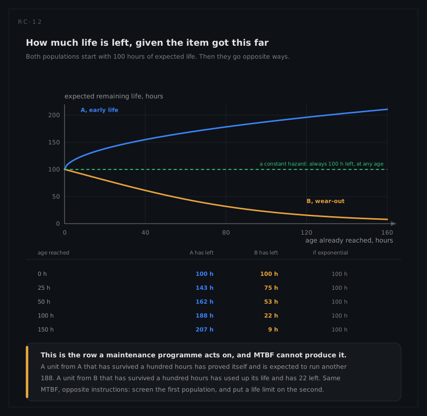
Not how long does it last, but it has got this far, what happens next. Conditional reliability over the next 25 hours:
| Survived to | A | B | If exponential |
|---|---|---|---|
| new | 0.575 | 0.997 | 0.779 |
| 25 h | 0.751 | 0.962 | 0.779 |
| 50 h | 0.793 | 0.844 | 0.779 |
| 75 h | 0.817 | 0.632 | 0.779 |
| 100 h | 0.833 | 0.380 | 0.779 |
| 125 h | 0.844 | 0.172 | 0.779 |
Same question as a duration, which is the mean residual life:
| Age reached | A has left | B has left | If exponential |
|---|---|---|---|
| new | 100 h | 100 h | 100 h |
| 25 h | 143 h | 75 h | 100 h |
| 50 h | 162 h | 53 h | 100 h |
| 100 h | 188 h | 22 h | 100 h |
| 150 h | 207 h | 9 h | 100 h |
Both columns start at the same 100 hours, because that is the mean life and the mean life is what MTBF measures. One row down, they have already parted. A unit of design A that has survived a hundred hours has proved itself and is expected to run another 188. A unit of design B that has survived a hundred hours has spent its life and has 22 left.
Two opposite instructions
| Design A, β below 1 | Design B, β above 1 | |
|---|---|---|
| What is failing | A defect present from new, in some of the units | Something that accumulates with age, in all of them |
| Scheduled replacement | Actively harmful. It swaps a proven unit for an unproven one | Applicable. The fit says at what age |
| What to do instead | Find the process escape; screen or burn in until it is found | Set a life limit against a tolerable failure fraction |
| What the fleet looks like later | Better than the average suggests, as the weak units leave | Worse than the average suggests, as the survivors age |
For design B the arithmetic of the life limit is direct, because it is just the B-life read at whatever failure fraction is tolerable:
| Replace at | Fraction that fails before getting there |
|---|---|
| 50 h | 4.1 per cent |
63 h, the B10 | 10 per cent |
| 70 h | 14.8 per cent |
| 80 h | 24.0 per cent |
For design A there is no such age, and the honest version of the burn-in option is unattractive:
| Burn-in | Batch scrapped | Survivors' R over the next 100 h |
|---|---|---|
| none | 0 | 0.279 |
| 12 h | 30 per cent | 0.365 |
| 24 h | 42 per cent | 0.402 |
| 48 h | 56 per cent | 0.452 |
Burning in for 48 hours throws away over half the batch to move reliability from 0.28 to 0.45. Screening is what you do while you find the defect, not instead of finding it. The value of the analysis here is not the burn-in table: it is that β below one, with an interval that excludes 1, says the problem is a manufacturing or process escape rather than a design life, and sends the investigation to a different place entirely.
What the shared MTBF would have cost
Had both reports been believed at face value and an exponential assumed, the same 100 hours would have produced one set of numbers for both designs:
| What MTBF = 100 h implies | A actually | B actually | |
|---|---|---|---|
B10 | 10.5 h | 1.6 h | 63.0 h |
B1 | 1.0 h | 0.03 h | 35.1 h |
| Median life | 69.3 h | 36.3 h | 100.9 h |
| Spread, sd of life | 100 h | 175 h | 28 h |
| Life left at 100 h | 100 h | 188 h | 22 h |
A B10 of 10.5 hours is wrong by a factor of 6.5 in one direction for design A and a factor of 6 in the other direction for design B. The quoted B1 for design A, 0.03 hours, is not a number to act on either: it sits an order of magnitude below the earliest observed failure and is pure extrapolation, which is the honest way to report it.
One qualification test, two datasets, one identical headline number, and two maintenance policies that have nothing in common.
Part two: the same analysis on field data
The clean case above had no survivors in it. Real data always does, and the survivors are usually most of it.
36 medium transport aircraft, two environmental control system packs each, 21,600 flight hours a year across the fleet. That is 600 flight hours a year for an average aircraft and 43,200 bearing-hours a year for the 72 installed packs, but the average hides a spread: the busiest tails fly close to twice it and the quietest about half, so bearing ages diverge even though the aircraft entered service together. Five years in, the FRACAS has enough removals of one item to fit a distribution to it, and the item is the one the RCM analysis gave a condition-based task to: the air cycle machine bearing. The removals only started arriving in numbers this year, which is why anybody looked.
The data, including the units that did not fail
Twenty bearings carry a confirmed disposition against this mode: thirteen failed by the degradation mode being analysed, and seven are suspensions, units still running at that age or taken off for some other reason. Ages in flight hours since installation:
| 1,180 s | 1,420 f | 1,655 s | 1,830 f | 2,010 s |
| 2,240 f | 2,390 f | 2,510 s | 2,680 f | 2,810 f |
| 2,950 s | 3,080 f | 3,210 f | 3,340 s | 3,480 f |
| 3,620 f | 3,750 s | 3,900 f | 4,080 f | 4,260 f |
The seven suspensions are not missing data and they are not failures. They are evidence that a bearing reached that age without failing, and throwing them away is the most common error in this analysis.
Fitting it two ways
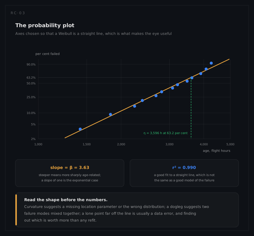
Median rank regression, with adjusted ranks for the suspensions and Bernard's approximation, and least squares of y on x as in part one:
β = 3.63 · η = 3,596 h · r² = 0.990
Maximum likelihood, on the same data:
β = 4.47 · η = 3,527 h
The two disagree about β by more than 20 per cent, and neither is wrong. Maximum likelihood is the better estimator asymptotically and is biased high for β on small samples; the correction is tabulated against the number of failures, and at thirteen the mean of β̂ ⁄ β is 1.124 against the 1.17 that applied to ten in part one, so dividing by it brings β to about 3.97. Rank regression is less efficient but more robust to a bad point, and it gives you the plot to look at. Report which method produced the number, because a β quoted without its method is not reproducible.
What throwing away the suspensions would have done
| β | η | |
|---|---|---|
| All 20 units, 13 failures and 7 suspensions | 4.47 | 3,527 h |
| The 13 failures only | 4.17 | 3,312 h |
The characteristic life comes out 6 per cent short. The direction is the point: discarding suspensions discards evidence of survival, so the fitted life can only get shorter, and every maintenance interval derived from it gets shorter with it. On a dataset with more suspensions than this one, the error runs to tens of per cent.
What the fit says
| Output | Value | What it means |
|---|---|---|
β | 4.47 | Strongly increasing hazard: a wear-out mode |
η | 3,527 h | The characteristic life, where 63.2 per cent have failed, whatever β is |
B10 | 2,131 h | Ten per cent have failed by this age |
B50 | 3,249 h | The median life |
| Mean life | 3,217 h | η · Γ(1 + 1/β), and not the same as η |
None of those is a number to submit on its own. From the same likelihood, by the Fisher matrix and on thirteen failures, the 90 per cent interval on β is 3.11 to 6.41 and on η it is 3,184 to 3,907 h. Then the B-lives, which are what a limit is actually set from:
| B-life | Point | 90 per cent interval | 90 per cent lower bound |
|---|---|---|---|
B10 | 2,131 h | 1,720 to 2,640 h | 1,803 h |
B5 | 1,814 h | 1,389 to 2,369 h | 1,473 h |
B1 | 1,259 h | 851 to 1,864 h | 928 h |
Read the last column, because a life limit is a one-sided question: nobody is harmed by the population turning out better than expected. The interval on β spans a factor of two and still clears 1 by a distance, so the wear-out finding survives its own uncertainty. The interval on B10 runs about a fifth below the point estimate and a quarter above it; the interval on B1 is a factor of two wide, which is the thin tail stated as a number rather than as a warning.
The hazard is the number that matters for maintenance, because it is what an age limit acts on:
| Age | Hazard |
|---|---|
| 1,000 h | 16 per 10⁶ h |
| 2,000 h | 177 per 10⁶ h |
| 3,000 h | 723 per 10⁶ h |
| 4,000 h | 1,959 per 10⁶ h |
The question maintenance actually asks
Not how long it lasts, but it has got this far, so what happens next? Conditional reliability over the next 500 flight hours:
| Survived to | R(next 500 h) |
|---|---|
| 1,500 h | 0.944 |
| 2,500 h | 0.763 |
| 3,500 h | 0.455 |
A bearing at 3,500 hours has a coin-toss chance of reaching 4,000. A bearing at 1,500 hours is almost certain to. No constant-rate model can say that, because under a constant rate all three rows are identical.
A variant with no failures at all
The same programme modified the bearing and put twelve modified packs into service. They have 900 flight hours each and no failures of this mode, and somebody wants to know what that proves. It is the Weibayes case: assume β = 4.47 from the unmodified population, and fit only η.
η = (Σ tᵢ^β ⁄ r)^(1⁄β) with r = 1 in place of the zero failures
Σ tᵢ^β = 12 × 900^4.47 = 1.93 × 10¹⁴ → η = 1,569 h, and dividing by −ln 0.10 = 2.303 instead of by 1 gives the 90 per cent lower bound, η ≥ 1,302 h.
Against the old design's 3,527 hours that proves nothing, and the reason is worth seeing rather than asserting: under the old distribution, twelve units at 900 hours would have been expected to produce 0.027 failures. Zero was the overwhelmingly likely outcome whether the modification worked or not. To demonstrate at 90 per cent confidence that the new bearing is at least as good as the old one, those twelve packs have to reach about 2,438 flight hours each with no failures, which at 600 hours a year is another two and a half years of flying. A wear-out life cannot be bought with early-life hours, and the Weibayes arithmetic is what says so before the trial is funded rather than after.
Reconciling with the constant rate everybody used
Every earlier analysis on this fleet carried 55 failures per 10⁶ hours for this item: the figure the prediction produced, years before there was field evidence to check it against. Over 43,200 bearing-hours a year that is 2.4 removals a year, and that is the demand the task analysis, the repair level analysis and the spares model were all sized on.
A fitted hazard cannot be compared with that directly, because one is a function of age and the other is not. What can be compared is the rate the fleet is generating now, and getting it needs the age profile as well as the fit.
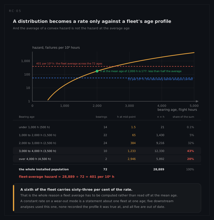
The 72 installed bearings, grouped by age:
| Bearing age | Bearings | Mid-point | h at the mid-point |
|---|---|---|---|
| under 1,000 h | 14 | 500 h | 1.5 per 10⁶ h |
| 1,000 to 2,000 h | 22 | 1,500 h | 65 per 10⁶ h |
| 2,000 to 3,000 h | 24 | 2,500 h | 384 per 10⁶ h |
| 3,000 to 4,000 h | 10 | 3,500 h | 1,233 per 10⁶ h |
| over 4,000 h | 2 | 4,500 h | 2,946 per 10⁶ h |
fleet-average hazard = Σ nᵢ h(tᵢ) ⁄ Σ nᵢ = 28,889 ⁄ 72 = 401 per 10⁶ h
Two things to notice before using it. The mean bearing age is 2,000 hours and h(2,000) = 177 per 10⁶ h, so the fleet average is more than twice the hazard at the mean age: the hazard is convex, and the twelve bearings past 3,000 hours contribute 63 per cent of the sum while making up a sixth of the fleet. Reading the hazard off at the mean age is the mistake this arithmetic exists to avoid.
The second is a temptation rather than a check. Running F across the same profile puts the expected failures at these ages at 13.2, which sits next to the 13 the FRACAS holds and looks like a validation of the fit. It is not one. These 72 bearings are the survivors, all of them alive at the age listed; the units that did fail were removed and their replacements sit in this same profile as young bearings, which is most of what the 14 under 1,000 hours are. Applying F to survivors' ages to recover failures those survivors did not have uses the population twice. The orders of magnitude agree, and that is all it says: a real check would have to run over the original cohort's exposure rather than over today's ages.
So the fleet is running at 401 per 10⁶ h, 7.3 times the 55 everything downstream carries, and 17.3 removals a year against 2.4. The fleet's own cumulative experience says the same thing more slowly: 13 failures in 216,000 bearing-hours, which is five years at 43,200 a year, is 60 per 10⁶ h averaged over the whole period. Already above the assumption, and that average is holding a rising number down.
That total is worth checking against itself, because a fleet cannot have flown more bearing-hours than it has flown. The 72 installed bearings carry 72 × 2,000 = 144,000 hours between them and the 13 that failed carried another 39,000 before they were removed, which is 183,000 bearing-hours accounted for. Five years of operation supplies 216,000, so the ages on this page fit inside the exposure that produced them with room to spare; four years would not have, and the arithmetic would have been describing a fleet that could not exist.
Forward, holding the fit and letting the fleet fly. Expected removals are counted rather than read off the current rate, and the quantity to count is the conditional one: every one of the 72 bearings is alive at its current age, so what a bearing of age aᵢ contributes over the next 600 hours is 1 − R(aᵢ + 600) ⁄ R(aᵢ), not F(aᵢ + 600) − F(aᵢ). That is the same distinction the hazard makes, given survival so far, and using the unconditional difference here understates the first year by nearly half.
Failures are replaced by new bearings, so each year the survivors age by 600 hours and the replacements re-enter at zero:
| Next | Expected removals | Against the plan |
|---|---|---|
| 600 flight hours | 16.8 | 2.4 |
| the 600 after that | 15.8 | 2.4 |
| the 600 after that | 14.1 | 2.4 |
The first row is the check that the arithmetic is right: 16.8 is what the current fleet-average hazard of 401 per 10⁶ h already implied, 17.3 a year. The sequence then falls, because the oldest bearings fail first and are replaced by new ones, which is the younger population the renewal creates.
A constant rate carried on a wear-out mode is a statement about one fleet at one age, and it expires quietly. Forty-seven removals over three years against the seven the support system was sized for, and nothing about the hardware changed. The constant was never a property of the item, so it could not carry a fleet forward, and every downstream analysis that used it inherited an expiry date nobody wrote down.
What has to change downstream
| Analysis | What this fit does to it |
|---|---|
| RCM | β > 1 with a definable age makes scheduled discard applicable, which it was not when the rate was assumed constant. A 5 per cent B-life sits at 1,814 h, with a 90 per cent lower bound of 1,473 h |
| Task analysis | The removal frequency, and therefore the workload, rises with fleet age |
| Level of repair | Demand is not 2.4 a year but about 17, and it keeps climbing, so the repair-level break-even moves with it |
| Prediction | The item's rate is age-dependent, so a single figure needs a stated age or a stated fleet |
| Spares | The pipeline sized on 2.4 a year is short by a factor of seven before anything else is decided |
That is the whole argument for doing this analysis: not the plot, and not β, but the fact that five downstream decisions were quietly resting on an assumption that twenty removal records can overturn.