

Four things to be clear about before fitting anything: what the distribution says, what the data has to look like, how the parameters get estimated, and how much to believe the answer.
The two-parameter Weibull
Everything in this module comes out of one function, the reliability: the chance that an item is still working at age t.
R(t) = e^(−(t⁄η)^β)
The other four follow from it by definition rather than by any further assumption, which is worth saying because they are often presented as five separate formulas to memorise.
| Formula | What it answers | |
|---|---|---|
| Reliability | R(t) = e^(−(t⁄η)^β) | What fraction is still working at age t |
| Unreliability, the CDF | F(t) = 1 − R(t) | What fraction has failed by age t |
| Density, the pdf | f(t) = (β⁄η)(t⁄η)^(β−1) e^(−(t⁄η)^β) | Where in time the failures fall |
| Hazard | h(t) = f(t) ⁄ R(t) = (β⁄η)(t⁄η)^(β−1) | The chance of failing next, given survival so far |
| Cumulative hazard | H(t) = (t⁄η)^β, so R(t) = e^(−H(t)) | The quantity the probability plot is built on |
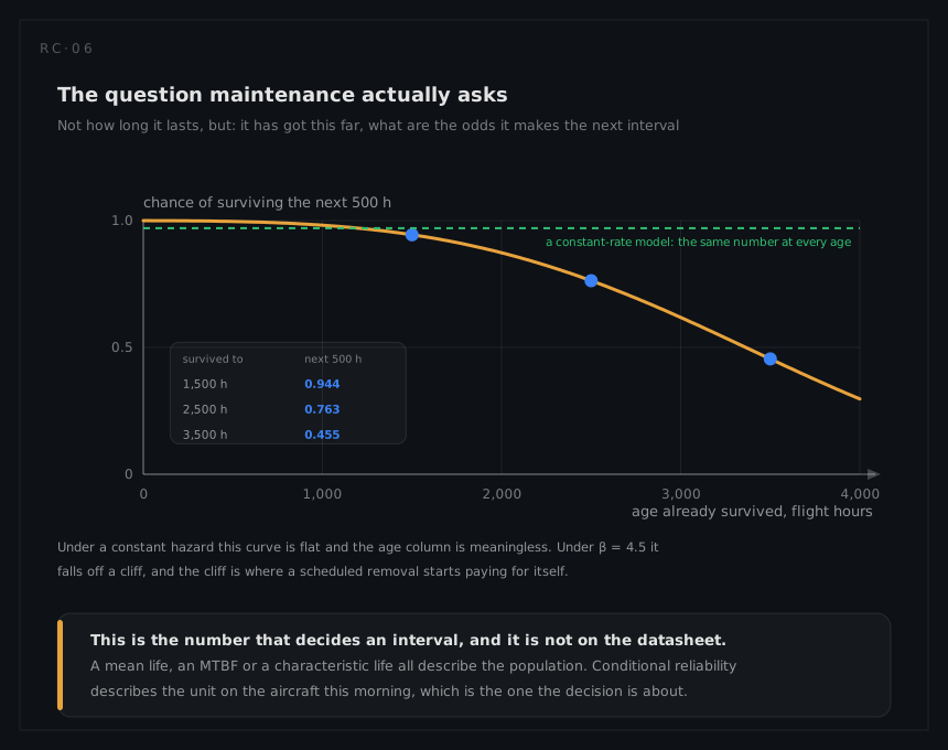
The hazard is the one that decides maintenance, and the phrase that makes it different from the other four is given survival so far. The density says how many of the original population fail around age t. The hazard says what the risk is for the unit that is on the aircraft this morning, having already survived. Only the second is a decision.
| Parameter | Name | What it does |
|---|---|---|
β | Shape | Decides whether the hazard falls, stays flat or rises with age |
η | Scale, the characteristic life | Sets where the distribution sits on the time axis |
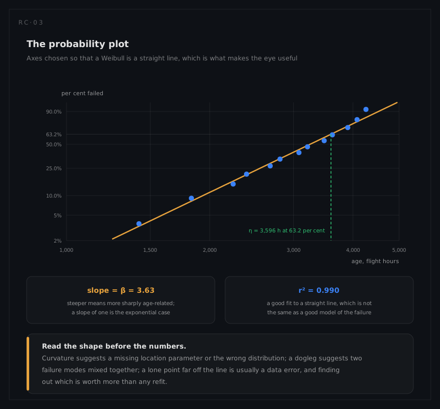
Two properties are worth memorising. At t = η, R = e⁻¹ = 0.368 whatever β is: 63.2 per cent have failed by the characteristic life, always, which is why the probability plot has a line ruled across it at that height. And β = 1 collapses the Weibull to the exponential, with η becoming the mean time between failures, so the constant-rate world is a special case of this one rather than a rival to it.
Getting a life out of the two parameters
β and η are not the answer to any engineering question. These are.
| Output | Formula | What it is for |
|---|---|---|
| B-life | Bp = η(−ln(1 − p))^(1⁄β) | The age by which a stated fraction p has failed: life limits, warranty, spares timing |
Median, B50 | η(ln 2)^(1⁄β) | The age half the population reaches |
| Mean life | η·Γ(1 + 1⁄β) | Costing, and the only honest comparison with a quoted MTBF |
| Variance | η²[Γ(1 + 2⁄β) − Γ(1 + 1⁄β)²] | How spread out the lives are, which MTBF hides completely |
| Mode | η((β−1)⁄β)^(1⁄β) for β > 1, and 0 otherwise | Where failures pile up, if they pile up anywhere |
| Conditional reliability | R(t + Δ) ⁄ R(t) | It got this far: will it make the next interval |
| Mean residual life | ∫R(u)du from t to ∞, over R(t) | How much life is left, given the age already reached |
The mean life is not η, and the gap between them is a function of β alone:
β | Γ(1 + 1⁄β) | mean ⁄ η | median ⁄ η | sd ⁄ mean |
|---|---|---|---|---|
| 0.5 | 2.000 | 2.000 | 0.480 | 2.24 |
| 1.0 | 1.000 | 1.000 | 0.693 | 1.00 |
| 2.0 | 0.886 | 0.886 | 0.833 | 0.52 |
| 3.5 | 0.900 | 0.900 | 0.901 | 0.32 |
| 5.0 | 0.918 | 0.918 | 0.929 | 0.23 |
| 8.0 | 0.942 | 0.942 | 0.955 | 0.15 |
Read the last column rather than the first. It is the coefficient of variation, and it is what separates a population you can put a life limit on from one you cannot. Two curiosities fall out of the table: Γ(1 + 1⁄β) bottoms out at 0.886, near β = 2.17, so for any β above 1 the mean life is within about 12 per cent of η; and near β = 3.44 the mean and the median coincide, because the distribution is very nearly symmetric there.
The third parameter, and when it is honest
The three-parameter form adds a location γ, a failure-free period before which nothing fails: R(t) = e^(−((t−γ)⁄η)^β).
It is legitimate when there is a physical reason for a failure-free period: a wear mechanism that has to remove material before anything can break, a corrosion process with an incubation time, a crack that has to reach a detectable size. It is not legitimate as a way to straighten a curved probability plot, which is what it is usually used for. A fitted γ with no mechanism behind it is a third degree of freedom bought with the data's credibility.
The data, including what did not fail
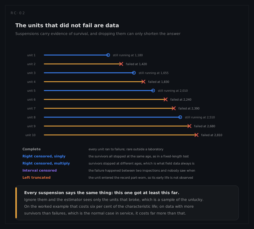
| Kind | What it means |
|---|---|
| Complete | Every unit ran to failure; rare outside a laboratory |
| Right censored, singly | The survivors all stopped at one age, as in a fixed-length test |
| Right censored, multiply | Survivors stopped at different ages, which is what field data always is |
| Interval censored | The failure happened between two inspections and nobody saw when |
| Left truncated | The unit entered the record part-worn, so its early life was never observed |
Four requirements on the data itself, and each one is a place where a dataset quietly stops being usable:
- Independent and identically distributed lives. This is the requirement the international standard states first, and the one field data breaks most often. The gaps between one repaired machine's successive failures are not a sample of lives: each interval begins from whatever state the last repair left behind. That is a process rather than a distribution, and it belongs to reliability growth and the NHPP models there.
- One failure mode per fit. A bearing that fails from grease breakdown and from cage fatigue is two populations, and a single fit describes neither.
- The right clock. Age has to be measured in whatever the damage accumulates with: hours, cycles, landings, starts, kilometres. A cyclic mode fitted against calendar time produces noise.
- Age since the mode was last renewed. For a repaired item, time since manufacture is the wrong origin unless the repair did nothing to the mode in question.
Estimating the parameters
Median rank regression
Sort the failures. Give each one a plotting position, an estimate of the unreliability at that order statistic. Bernard's approximation is the standard shortcut, accurate enough that the exact median rank is almost never worth computing:
F(i) ≈ (i − 0.3) ⁄ (N + 0.4)
Then straighten the model. Take logs of R(t) = e^(−(t⁄η)^β) twice and it becomes a straight line:
ln(−ln(1 − F)) = β·ln t − β·ln η
So plotting y = ln(−ln(1−F)) against x = ln t gives a line whose slope is β and whose intercept is −β ln η. Least squares on those N points is the estimate. Two details that change the answer and are usually left unstated: practitioner software regresses x on y rather than y on x, on the argument that the recorded age carries the error and the plotting position does not, and the two directions disagree by a per cent or two on good data and more on bad.
Suspensions get no plotting position of their own. What they do is push the later failures down the rank order, through an adjusted rank with increment
I = (N + 1 − previous adjusted rank) ⁄ (1 + units remaining, counting this one)
with each failure's adjusted rank being the previous one plus I. With no suspensions the increment is exactly 1 and the ranks are 1, 2, 3 and so on, which is the check that the formula is being applied correctly.
Maximum likelihood
Choose the β and η that make the observed data likeliest. Differentiating the log-likelihood and setting both derivatives to zero eliminates η and leaves a single equation in β:
Σtᵢ^β ln tᵢ ⁄ Σtᵢ^β − 1⁄β = (1⁄r)·Σ ln tᵢ
solved numerically, and then η = (Σtᵢ^β ⁄ r)^(1⁄β). With suspensions in the data the tᵢ^β sums run over every unit, the ln tᵢ sum runs over the failures only, and r is the number of failures. That asymmetry is the whole of how the method uses a survivor: it contributes its exposure and not its death.
| Rank regression | Maximum likelihood | |
|---|---|---|
| Gives you | A plot to look at | The efficient estimate |
| Small samples | More stable, less efficient | Biased high in β, correctably |
| Robustness | Less sensitive to one bad point | Sensitive, because every point enters the likelihood |
| Heavy censoring | Degrades as suspensions dominate | Handles it properly |

The small-sample bias, and the interval
A maximum-likelihood β on a dozen failures is too big, systematically. The useful fact is that for a complete sample the distribution of β̂ ⁄ β depends on the sample size and on nothing else: not on the true β, not on η. That single property gives both the correction and the confidence interval, and it is why the unbiasing tables in the literature can be reproduced by anyone with a random number generator.
For ten complete failures the mean of β̂ ⁄ β is about 1.17, so an estimate of 4.0 corresponds to a β of about 3.4. The fifth and ninety-fifth percentiles are about 0.74 and 1.82, so a 90 per cent interval runs from β̂⁄1.82 to β̂⁄0.74: a factor of two and a half wide. Ten failures is a normal amount of data and a small amount of evidence, and both statements have to survive into the report.
An interval on the B-life, not only on β
An interval on β settles whether the mode is age-related. It does not settle the number anybody is actually going to sign, which is a life limit, and a B-life needs its own bound. Two routes are in general use and the international standard carries both.
- Fisher matrix. Invert the observed information from the likelihood to get the variances of
β̂andη̂and the covariance between them, then propagate to whatever is wanted. For a B-life the propagation is one line, becauseln Bp = ln η + (1⁄β)·ln(−ln(1 − p))is nearly linear in the two parameters: take the variance of that expression and set the bound on the log scale, so it cannot come out negative. It is quick, it works with censoring, and it is an asymptotic approximation that gets optimistic on very small samples. - Beta-binomial bounds on the rank regression. Instead of the parameters, put a bound on each plotting position: the
i-th ofNorder statistics has a known beta distribution, so the 5th and 95th percentiles of each rank give a band around the fitted line, read off at whatever failure fraction the decision needs. This is the route that pairs with a probability plot, because the bound is drawn on the plot.
Two properties are worth knowing before either is quoted. The bound is one-sided for a life limit: nobody is harmed by the population being better than expected, so the number to report is the lower bound, not the width of a two-sided interval. And the bound widens fast into the tail: on the worked example's thirteen failures the 90 per cent interval on B50 is ±10 per cent, on B10 about a fifth below and a quarter above, and on B1 a factor of two. That widening is the honest statement of how far the fit can be extrapolated.
Weibayes
Sometimes called the one-parameter Weibull: assume β from experience with the same mechanism and fit only η. It exists for the case that comes up constantly in service, a handful of failures or none at all and a decision that has to be made anyway. It is not a shortcut somebody invented: the international standard carries it in a normative clause, and it appears normatively in component standards too. Its answer is exactly as good as the assumed β, which is why the assumption is stated rather than buried. The worked example runs the arithmetic on a modified bearing with no failures at all, which is the case it was invented for.
What a mean life does not tell you
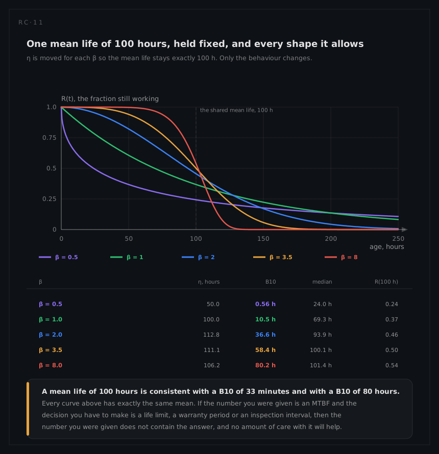
An MTBF is the mean of the distribution and nothing more. Hold it fixed at 100 hours and move β, adjusting η to compensate, and the population goes from one where a tenth is dead inside an hour to one where a tenth survives to 80 hours.
Every curve in that figure has the same mean. If the number you have been given is an MTBF and the decision in front of you is a life limit, an inspection interval, a warranty period or a spares buy, the number does not contain the answer, and no amount of care in using it will put the answer back. That is not a criticism of MTBF; it is a statement about which question it answers. The worked example takes two real datasets that produce the same 100 hours and follows the consequences all the way to two opposite maintenance policies.
How much to believe it
- The plot before the statistic. Curvature suggests a missing location parameter or the wrong distribution; a dogleg suggests two modes; a lone outlier is usually a data error, and finding out which is worth more than any refit.
r²is not validation. A high correlation means the points lie near a line. It says nothing about whether the line is the right model where the decision is being made.- Confidence intervals are not optional on small samples. With ten or fifteen failures the interval on β routinely spans a factor of two, which is the difference between wear-out with a removal to schedule and random with nothing to do.
- The tails are the weakest part. A B1 life extrapolated from thirteen failures, none of them early, is an extrapolation into the region with no data.
What to use instead of r²
Saying twice that r² is not validation is only half an answer. Three things are, in ascending order of formality.
- The residual pattern. Not how far the points sit from the line but where: a systematic bow, a dogleg, or a run of points on one side is a statement about the model, and the eye is better at it than any single statistic. Do this one first, always.
- A formal goodness-of-fit test. The international standard carries the tests appropriate to Weibull data, including the case where the parameters were estimated from the same sample, which is what makes the ordinary tabulated critical values wrong. Report the test and its significance level, not just the word passed.
- A comparison against the alternative. Goodness of fit answers is the Weibull tolerable; it does not answer is the Weibull better than the lognormal, which is usually the live question. Fit both by maximum likelihood and compare the log-likelihoods, with a penalty for parameters if the two models do not have the same number. If the two are close, the honest report says the data cannot separate them, and then it says whether the decision differs between them: often it does not, and the argument was never worth having.
One caution that applies to all three. A test that passes is not a licence to extrapolate. Goodness of fit is judged where the data is, and a life limit is usually set where it is not.
The outputs that get used
| Output | Definition | Used for |
|---|---|---|
B10, B50 | The age by which 10 or 50 per cent have failed | Life limits, warranty periods, spares timing |
Characteristic life η | 63.2 per cent failed | Comparing designs and populations |
| Mean life | η Γ(1 + 1⁄β) | Costing, and comparison with an assumed MTBF |
| Hazard at an age | h(t) | The failure rate to hand to a model, at a stated age |
| Conditional reliability | R(t + Δ) ⁄ R(t) | The maintenance question: it got this far, will it make the next interval |
| Mean residual life | Expected life remaining at age t | The same question asked as a duration rather than a probability |
What the fit does to everything else
A fitted β above one means the item's failure rate is a function of the fleet's age profile, not a property of the item. Every downstream model that holds a single rate is then carrying a snapshot with an expiry date:

That is the real product of this analysis. Not the plot, and not β, but the discovery that a number several other analyses depend on was true at one moment and is quietly ageing out of date.