

The deliverable is two parameters and a plot. What makes it useful is everything reported around them.
1. The fit, with its provenance
| Field | Why it travels with the numbers |
|---|---|
| β and η | The fit itself |
| The estimator | Rank regression and maximum likelihood disagree, routinely by twenty per cent in β |
| Failures and suspensions | Thirteen failures and seven suspensions is a different claim from twenty failures |
| The confidence interval on β | On small samples it spans a factor of two, and the decision may not survive it |
| The failure mode | A fit to a mixture describes nothing |
| The clock and the origin | Hours or cycles, since manufacture or since the last renewal |
A β quoted without those six is not reproducible and cannot be reviewed.
2. The engineering answer
| Output | The worked example |
|---|---|
| Shape | β = 4.47: strongly age-related, a wear-out mode |
| Characteristic life | η = 3,527 h |
| B10 | 2,131 h, with a 90 per cent lower bound of 1,803 h |
| Median life | 3,249 h |
| Conditional reliability over 500 h | 0.944 at 1,500 h, 0.455 at 3,500 h |
The conditional reliability row is the one maintenance uses. The others describe the population; that one describes the unit on the aircraft this morning.
3. A mean life, if anyone asks for one, with what it hides beside it
A fit can always be collapsed to a single mean, and somebody will want it for a cost model. Report it with the two numbers that stop it being read as a description of the item's life:
| Alongside the mean | Why |
|---|---|
| β | The mean is compatible with almost any failure behaviour; β is what says which one this is |
The spread, as a standard deviation or a B10 | Two populations with the same mean can have B10 lives a factor of forty apart |
The worked example's first half is exactly that case: two datasets, both ten failures in a thousand hours, both a mean life of 100 hours, B10 lives of 1.6 h and 63 h, and opposite maintenance policies. A mean life quoted on its own would have been true about both and useful about neither.
4. What the fit invalidates
| Analysis | What it inherits |
|---|---|
| Prediction | The item's rate is now a function of age, and any single figure needs an age attached |
| RCM | β > 1 makes scheduled restoration and discard applicable; the decision reopens |
| Fault tree and RBD | Basic event rates that were assumed constant |
| LORA and spares | Demand that rises with fleet age, and break-evens that move with it |
| Maintenance intervals | Any interval derived from a constant hazard on this mode |
5. What to watch, and when to refit
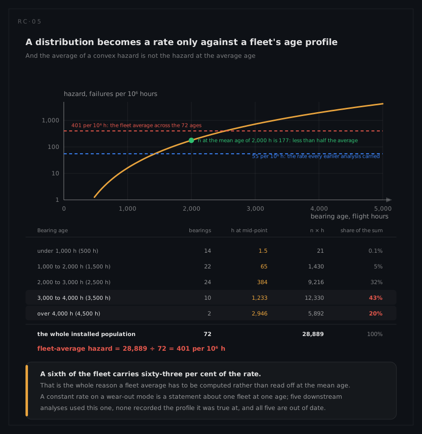
The fleet's own age profile against the fitted distribution: how much of the population is approaching the region where the hazard climbs, and when the next tranche gets there. That is a forecast the fit produces for free, and it is the trigger for the next review.
What the results do not support
- They are not a prediction for a different fleet. A different duty cycle, environment or operator changes the distribution, and the parameters do not transfer without an argument.
- They do not extrapolate safely. A B1 life from thirteen failures, none of them early, sits in a region with no data and a very wide interval.
- They do not describe a mixture. Two competing modes need two fits, and a single fit across both is a curve nobody should act on.
- They are not permanent. Every year of service adds data where the current fit is weakest, and the refit is not optional maintenance of a document: it is the analysis catching up with the fleet.
- They do not justify an age limit on their own.
β > 1makes an age-based task applicable; whether it is effective is a cost or a risk question, and it belongs to RCM.