

The same environmental control system pack, three years earlier: a development test programme before the fleet existed. The requirement is 500 hours MTBF at entry into service; the first prototype is nowhere near it. Every value is an illustrative teaching figure.
The test
A time-terminated test of 5,000 accumulated pack hours with test-analyse-and-fix between incidents. Eighteen relevant failures, at these cumulative test times:
62 · 118 · 214 · 340 · 470 · 615 · 830 · 1,045 · 1,290 · 1,620 · 1,970 · 2,340 · 2,760 · 3,180 · 3,610 · 4,080 · 4,520 · 4,930
Read the gaps rather than the times. The first six failures arrive in the first 615 hours; the last six take 2,590 hours between them, counting from the failure before them. That widening is the growth, and everything that follows is a way of putting a number on it.

The Duane fit, for the eye

Cumulative MTBF at the ith failure is just tᵢ ⁄ i: 62 hours at the first, 59 at the second, 71 at the third, and so on up to 274 at the eighteenth. Logging both axes and running least squares on the eighteen points gives
α = 0.389 · r² = 0.968
and with it the relationship the plot exists to support:
instantaneous MTBF = cumulative MTBF ÷ (1 − α)
On this slope that factor is 1 ÷ 0.611 = 1.64, which would put the end-of-test instantaneous MTBF at 455 hours. The figure reported later in this chapter is 427, from the likelihood fit and its β̂. The two are close, and the second one is the estimate: the plot's slope has no standard error worth the name behind it.
That r² deserves no weight at all. The point at the fifth failure contains all the data in the first four, so the eighteen points are heavily correlated and a regression's standard errors do not apply to them. The plot is a diagnostic and not an estimator, and its job here is to answer one question by eye: is the line rising?
The Crow-AMSAA fit, for the number
For a time-terminated test with n failures at times tᵢ ending at T:
β̂ = n ÷ Σ ln(T ⁄ tᵢ) and λ̂ = n ⁄ T^β̂
The sum is the whole calculation. ln(5000⁄62) = 4.390, ln(5000⁄118) = 3.747, down to ln(5000⁄4930) = 0.014, and the eighteen terms add to 27.661. So
β̂ = 18 ÷ 27.661 = 0.651 and λ̂ = 18 ÷ 5000^0.651 = 7.05 × 10⁻²
β below one means the failure intensity is falling, which is what growth is.
Correcting it, and putting an interval on it
β̂ is biased high, exactly, by n⁄(n−1). On eighteen failures that is 18/17, so
β̄ = (17⁄18) × 0.651 = 0.615 and α = 1 − β̄ = 0.385
Which puts the two methods within four thousandths of each other: 0.385 from the corrected likelihood against 0.389 from the plot. The disagreement the uncorrected numbers showed, 0.35 against 0.39, was almost entirely one estimator reporting a known bias. That agreement is not guaranteed on every dataset, but the bias is, and correcting for it is not optional.
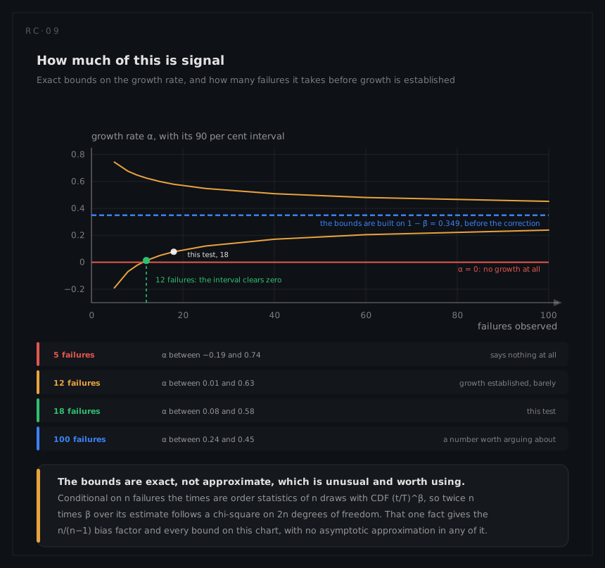
The interval comes from the same fact. With 2nβ⁄β̂ distributed as a chi-square on 36 degrees of freedom, and χ²(0.05, 36) = 23.27, χ²(0.95, 36) = 51.00:
| Value | 90 per cent interval | |
|---|---|---|
β | 0.651, corrected to 0.615 | 0.42 to 0.92 |
α | 0.385 | 0.08 to 0.58 |
Those bounds are built on the uncorrected β̂, because that is what the chi-square pivot contains: the correction moves the point estimate, not the interval. So the reported α of 0.385 does not sit at the centre of 0.08 to 0.58, and it is not supposed to.
The exactness stops there. The obvious next move is to push the two β bounds through T⁄(nβ) and quote 301 to 660 hours as a 90 per cent interval on the instantaneous MTBF. It is not one. That substitution holds the observed count of eighteen fixed as though it were the expected count, so it drops the Poisson variation in the count entirely; simulating the fitted process shows the range it produces covers the true MTBF about 75 per cent of the time, not 90. An interval on instantaneous MTBF needs bound factors derived for MTBF itself. The bounds on β and α are exact and they do not transfer, so 427 hours is reported here as a point estimate with the α interval beside it.
That interval on α is the honest headline, and it is wide. It still clears zero, so growth has been demonstrated; at this growth rate it would have taken twelve failures to get that far, and this test has eighteen. What the interval does not support is an argument about whether α is 0.35 or 0.39, which is what the first draft of this analysis spent its time on.
Does the power law fit these failures

The Cramér-von Mises statistic on this data is C² = 0.014, against a 10 per cent critical value of about 0.17 for eighteen failures. Not rejected, and comfortably so. Two honest caveats travel with that:
- These are illustrative teaching times, and they lie closer to a smooth power law than a real test would. On real data the statistic will be larger.
- The test is weak at this sample size. A programme whose intensity steps at a design review, rather than falling continuously, can walk straight through it: a step from 179 hours MTBF to 625 is caught a little over four times in ten at that same 10 per cent value, and it takes a step out to 2,500 hours before the test catches four in five. The right-hand panel above is exactly that case: the points bow away from the diagonal, its Duane
r²is 0.70 against 0.968, and the formal test passes it anyway.
Which estimator, and what the alternatives would have given

| If the test had been | β̂ | Correction | Instantaneous MTBF |
|---|---|---|---|
| Time-terminated at 5,000 h, exact times | 0.651 | (n−1)⁄n, 5.9 per cent | 427 h |
| Failure-terminated at the 18th failure | 0.657 | (n−2)⁄n, 12.5 per cent | 417 h |
| Recorded as five interval counts | 0.589 | 472 h |
The middle row is the trap. The same eighteen times, stopped by a different rule, need a correction more than twice as large, and nothing in the data announces which rule applied. The test type is a property of the test plan, not of the failure times, and if it was not written down it cannot be recovered.
Where the design actually was
| Test hours | Cumulative MTBF | Instantaneous MTBF |
|---|---|---|
| 250 | 98 h | 150 h |
| 1,000 | 158 h | 243 h |
| 2,000 | 202 h | 310 h |
| 3,000 | 232 h | 357 h |
| 5,000 | 278 h | 427 h |
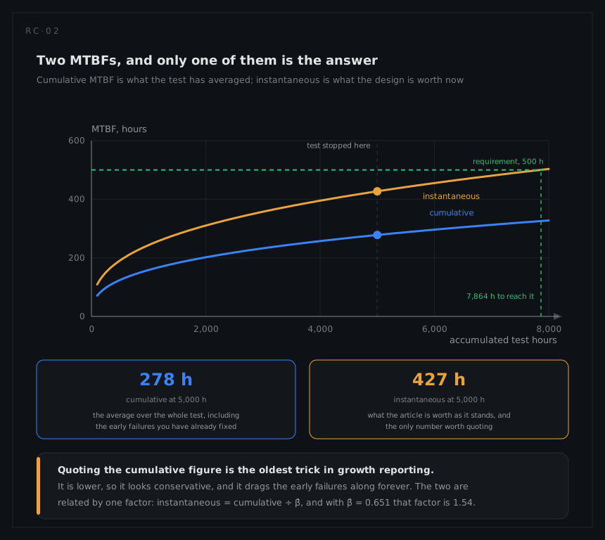
Both columns are one division apart, and at the end of the test the arithmetic needs no model at all: cumulative MTBF is T⁄n = 5,000⁄18 = 278 h, and instantaneous is T⁄(n β̂) = 5,000⁄(18 × 0.651) = 427 h. They differ by exactly 1⁄β̂, which is 1.54 here.
Quoting 278 hours at the end of that test would be wrong, and it is the most common misreport in the field. The cumulative figure carries the early failures forever, including the ones that were designed out at hour 300. What the article is worth on the day the test stops is 427 hours.
Reaching the requirement
m(t) = t^(1−β) ⁄ (λ β), so t = (m · λ · β)^(1 ⁄ (1−β))
For 500 hours: 7,864 accumulated test hours, which is 2,864 more than the test has run. At twenty test hours a day, five days a week, that is another six and a half months, on top of the eleven and a half already spent, and every fix inside it has to be designed, made, fitted and re-tested.
That is the arithmetic programmes discover late. The curve flattens as it rises, so every hour of MTBF near the target costs more test time than any hour before it: the last 73 hours, from 427 to 500, need 39 test hours each, against 16 test hours each for the 318 hours of MTBF the first 5,000 test hours bought.
The ceiling

More test time cannot help beyond a limit set by two decisions:
growth potential = 1 ÷ (λA + (1 − d) λB)
where λA is the intensity of the modes nobody intends to fix and d is how effective the fixes to the rest turn out to be. On this programme the early intensity is 9.19 × 10⁻³ per hour, an MTBF of 109 hours:
| A-modes | Fix effectiveness | Growth potential | Against a 500 h target |
|---|---|---|---|
| 5% | 0.9 | 751 h | reachable |
| 5% | 0.7 | 325 h | unreachable by testing |
| 15% | 0.9 | 463 h | unreachable by testing |
| 25% | 0.8 | 272 h | unreachable by testing |
Same test, same failures, same effort. The difference between the first row and the third is how many modes the programme decided not to fix, and that decision is worth more than the test schedule.
What a projection says
Tracking says where the design is; the ceiling says how far it could ever go. Projection answers the question between them: where the design lands once fixes that have been identified but not yet embodied are actually in the hardware. It is the only one of the three activities that predicts, and it needs a programme shape this test did not have, so take a second article: the same 5,000 hours run as test-find-test, with every fix held back to one corrective action period at the end.
Nothing is embodied while it runs, so the intensity does not fall. It stays at the 9.19 × 10⁻³ per hour this design starts at, and 5,000 hours produce 46 failures rather than eighteen. They belong to twenty-one distinct modes:
| Mode class | Distinct modes | Failures | Rate per hour |
|---|---|---|---|
| A, nobody intends to fix | 4 | 5 | λA = 1.00 × 10⁻³ |
| B, fixes designed in the corrective action period | 17 | 41 | λB = 8.20 × 10⁻³ |
Individual fix effectiveness runs from 0.60 on a supplier part nobody controls to 0.95 on a software change, weighting out to d̄ = 0.90 across the 41 failures. The projected intensity is three terms:
ρ_proj = λA + Σ (1 − dᵢ) λBᵢ + d̄ · h(T)
The middle term is what imperfect fixes leave behind, and because d̄ is the failure-weighted mean it collapses to (1 − d̄) λB. The last term is the allowance for modes nobody has seen yet, and it is the term that makes this a prediction rather than a recalculation. Fitting the same power law to the 17 times at which a new B-mode first appeared gives a discovery exponent of βd = 0.30, and for that fit h(T) = m βd ⁄ T exactly, so 17 × 0.30 ⁄ 5,000 = 1.02 × 10⁻³: one new mode roughly every 980 hours, still arriving at the end of the test.
| Term | Per hour | What it is |
|---|---|---|
λA | 1.00 × 10⁻³ | the modes nobody will fix |
(1 − d̄) λB | 8.20 × 10⁻⁴ | what imperfect fixes leave behind |
d̄ · h(T) | 9.18 × 10⁻⁴ | the modes not yet seen, fixed as well as the rest |
ρ_proj | 2.74 × 10⁻³ | projected MTBF 365 h |
Read that against the ceiling, and read the ceiling carefully. These 46 failures put 1.00 × 10⁻³ of a total 9.20 × 10⁻³ into A-modes: eleven per cent, not the five per cent the first row of the table above assumed. At the same d = 0.9 this article's growth potential is therefore 1 ÷ 1.82 × 10⁻³, or 549 hours, sitting between the 751 of that row and the 463 of the fifteen per cent one. The requirement is still reachable in principle, and the two hundred hours between 751 and 549 came from one judgement about which modes get fixed, not from anything the test did. The projection says the corrective action period gets to 365, and the whole of the difference between the two intensities is the third term, which is 34 per cent of the projected intensity. Leaving it out is how a projection turns into an argument that the requirement has already been met.
What the fleet then did

| MTBF | |
|---|---|
| Start of test | 109 h |
| End of test, instantaneous | 427 h |
| Requirement | 500 h |
Growth potential, at 5 per cent A-modes and d = 0.9 | 751 h |
| The fleet, in service | 1,667 h |
The fielded pack runs at nearly four times the end-of-test figure. That fleet number is the seven operational-consequence modes the RCM analysis lists for this same pack, 600 failures per 10⁶ hours between them; the two safety-consequence modes there are largely held off by scheduled tasks rather than counted as failures in service. Four reasons for the gap, none of them statistical: growth did not stop at entry into service, production hardware is not prototype hardware, the test environment was deliberately harsher than the real one, and the test counted incidents the fleet does not record as failures.
The direction is not predictable. Programmes where the field turns out worse than the test are at least as common, usually because the test environment was gentler than the world. A growth result is evidence about a test, not a promise about a fleet, and the only thing that settles the argument is service data.