

Nine steps. The first three happen before any hardware runs, and they are the ones that decide whether the programme can succeed at all.
1. Establish where the design starts
An initial MTBF, from the prediction, from a previous programme, or from the first hours of test. It will be optimistic, and everybody knows it is optimistic; what matters is that the number is written down, because the whole plan is measured against it.
2. Compute the ceiling before planning the curve
growth potential = 1 ⁄ (λA + (1 − d) λB)
Two judgements: what fraction of the intensity belongs to modes nobody will fix, and how effective the fixes will actually be. If the requirement is above the growth potential, stop and change the design, because no test plan reaches it. This step costs an afternoon and it is routinely skipped until the money is spent.
3. Draw the planning curve, and treat it as a budget
An idealised curve from the initial MTBF to the requirement, with the test time it implies and the management strategy behind it: how quickly fixes are designed and embodied, how many corrective action periods there are, and what fraction of the intensity the programme intends to address at all, MS = λB ⁄ (λA + λB). A planning curve is a budget and can be set to an impossible number, so it is reviewed against step 2 rather than against optimism.
4. Set the failure classification rules first
Relevant or not, chargeable or not, A-mode or B-mode. Written and agreed before the test, exactly as in FRACAS, because afterwards every classification is an argument with a growth rate attached. This is the single largest source of dishonest growth curves.
5. Run the loop, and keep it short
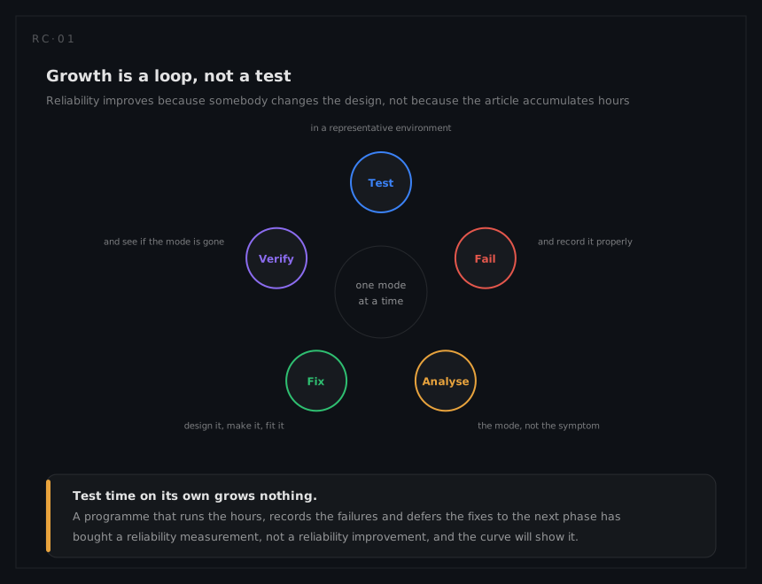
The rate of growth is set by how fast the loop turns. Deferring fixes to a later build is a legitimate management strategy, and its consequence is that the intensity does not fall during this test, which the model will report faithfully.
6. Track with the estimator, diagnose with the plot

Fit the power law process by maximum likelihood, and match the estimator to the test type. The formula for β̂ is the same either way; the bias correction and the bounds are not, and on eighteen failures the two corrections are 5.9 per cent and 12.5 per cent.
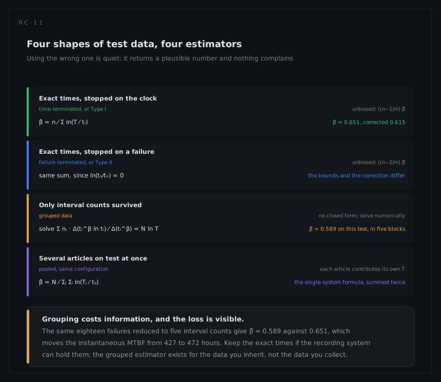
Then apply the correction, because it is exact rather than approximate:
β̄ = ((n−1)⁄n)·β̂ time-terminated, ((n−2)⁄n)·β̂ failure-terminated
Report:
| Quantity | Note |
|---|---|
| β̄, corrected, and α = 1 − β̄ | Say which correction and which test type |
| The interval on α | From 2nβ⁄β̂ ~ χ²(2n); exact, and wider than anyone expects |
| Instantaneous MTBF at the current time | T⁄(n β̂) at the end of test, the answer to where the design is |
| Cumulative MTBF | Alongside, never instead |
| Goodness of fit | With the caveat that the test is weak below a few dozen failures |
7. Project across corrective action periods
Where fixes have been identified but not yet embodied, projection estimates where the design will be once they are, using the expected effectiveness of each:
ρ_proj = λA + Σ (1 − dᵢ) λBᵢ + d̄ · h(T)
The modes nobody will fix, plus what imperfect fixes leave behind, plus an allowance for the modes not yet seen, taken from the rate at which new modes are still being discovered at T. It is the only one of the three activities that predicts, it inherits the honesty of the effectiveness estimates, and the third term is the one that gets quietly dropped: the worked example shows what dropping it does.
8. Answer the schedule question with arithmetic
t = (m · λ · β)^(1 ⁄ (1 − β))
gives the accumulated test time to reach an MTBF of m. Because the curve flattens as it rises, every hour of MTBF near the target costs more test time than any hour before it: on the worked example, going from 427 to 500 hours takes another 2,864 test hours on top of the 5,000 already run, which is 39 test hours for each hour of MTBF against 16 over the test so far.
9. Close the loop with the field
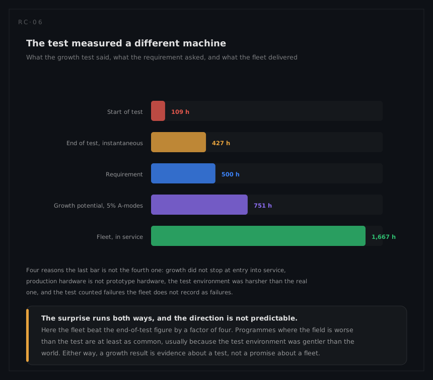
When service data arrives, put the observed rate beside the end-of-test figure and explain the difference: environment, build standard, duty cycle, counting rules. That comparison is the only validation a growth model ever receives, and a programme that never performs it has no evidence that its method works.