End-to-End Industry Examples

Availability is the property that will not stay inside the design office. This chapter takes eight systems, one from each industry the platform serves, and works the availability question on each of them: what the ledger counts as downtime, which hours belong to the design and which to the support system, what the denominator should be when clock time is the wrong measure, and what the resulting number tells someone to buy, schedule or re-write. The arithmetic is the same in all eight; what changes, sharply, is where the downtime actually comes from.

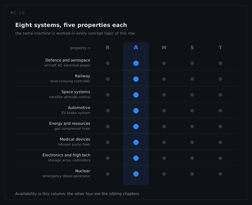
The eight systems are the same in every concept topic of this row. The aircraft electrical system worked here for its dispatch and its logistics tail is the one worked in reliability for its failure rates, in maintainability for its repair times, in safety for its catastrophic failure condition and in testability for its built-in test coverage. Read a column and you learn one property across eight industries; read a row and you watch one machine reveal its five RAMS faces. Every value below is illustrative: invented for teaching, chosen to be plausible and to make the arithmetic legible, and none of it is field data from any real product.

Defence and aerospace: aircraft electrical power

Two engine-driven integrated drive generators, an APU generator, a ram air turbine and the control units and contactors between them. The availability question is not whether the electrical system works, because it almost always does; it is whether the aeroplane can be dispatched this morning, and where the spare generator happens to be sitting when it cannot.

Convert both availabilities into hours and the gap becomes an object you can argue about. Inherent unavailability is 9 × 10⁻⁴, which at 3,000 flight hours a year is 2.7 hours; operational unavailability is 3.8 × 10⁻³, or 11.4 hours. The design delivers the first number and the support network spends the other 8.7 hours, a factor of 4.2 applied to a machine nobody touched. The single line item that does it is visible in the same table: an IDG removal at an outstation carries 26 hours of waiting on top of 1.5 hours of work, so wrench time is 5.5% of the event and the spare's location is the other 94.5%. The Ai-to-Ao decomposition exists to make exactly this attribution possible, and it settles the usual argument before it starts: no achievable improvement in generator failure rate closes an 8.7-hour gap that contains almost no repair.

The second lesson is the one aviation contributes that no other row does. Dispatch is permitted with one IDG inoperative for up to three days, and that provision breaks the assumed link between "failed" and "unavailable". The fault is open, the removal is scheduled, and the aeroplane is still earning. Availability here is bought partly with a rule rather than with hardware or with stock, and the rule is only affordable because the redundancy is genuine: the allowance is drawn against the margin the safety analysis proved, which is why its length is negotiated with certification rather than with operations. Treat it as free capacity and the availability gain has been taken out of the safety case without anyone recording the withdrawal.

Both observations point the same way when the money is allocated. Of the three availability levers, the design lever is nearly exhausted on this system and the support lever is barely used. Forward-positioning one IDG at the busiest outstation attacks 26 hours per event directly; a component improvement programme attacks 1.5.

Railway: level-crossing controller

A crossing sits on the network's critical path and can only be worked on when no trains are running. Everything distinctive about its availability follows from that one sentence.

The numbers close on themselves neatly. Operational unavailability of 1.82 × 10⁻³ over 8,760 hours is 15.9 hours per crossing-year, and across 40 crossings that is the 638 crossing-hours the fleet reports. Notice also that 9.5 divided by 2.5 is 3.8, and 1.82 × 10⁻³ divided by 4.8 × 10⁻⁴ is 3.79: the failure rate has cancelled out. When the same events are being counted in both ledgers, the ratio of the two availabilities is nothing more than the ratio of the two downtimes, which is why an Ai-to-Ao gap can always be read directly as a statement about delay and never needs a reliability argument to explain it.

What fills the seven hours between active repair and mean downtime is not a spare in a warehouse. It is access: the technician is ready, the part is in the van, and the track is occupied until the night possession. In the ledger this behaves exactly like logistics delay, but it responds to completely different money. Buying stock does nothing; what helps is batching work so that one possession clears several faults (maintenance task analysis run on a possession window rather than on a single job), remote diagnosis good enough that the right part travels on the first visit, and, at design time, moving as much of the equipment as possible to positions reachable without a possession at all.

One quiet point of bookkeeping is worth extracting, because it catches people. The inherent downtime of 4.2 hours a crossing-year at 2.5 hours an event implies only about 1.7 outage events a year, while the reliability column counts roughly 17 failures a crossing-year from the same equipment. The two are not in conflict: the availability ledger counts events that take the crossing out of service, and the reliability ledger counts failures, most of which are one lamp of four or a fault cleared inside a routine visit. A programme that quietly swaps one population for the other will produce an availability forecast wrong by an order of magnitude, in whichever direction suits the author.

Space systems: satellite attitude control

Seven years in orbit, no repair, and an availability figure that is not about the spacecraft being alive but about whether it was pointing correctly when the ground station asked for an image.

The denominator is the first thing to notice. This system's availability is quoted against imaging service, not against clock time and not against "spacecraft healthy", and it has to be, because the payload is scheduled for only 22% of orbit time and a fault during an eclipse pass may cost nothing at all. Choosing the denominator is a real engineering act here rather than a reporting convention: the same 45 hours of safe mode a year (2.5 entries at 18 hours) is charged as 0.51 percentage points against the imaging account, and would look quite different measured any other way. Subtract that from the 1.7 points of total unavailability behind Ao = 0.983 and about 1.2 points remain, owned by everything else in the chain that stands between an ordered image and a delivered one.

The restoration line is where the space row separates itself from every repairable system in this chapter. Mean restoration is 7.2 hours and the safe-mode event is charged at 18, so roughly 10.8 hours of each outage is time during which nobody is doing anything to the spacecraft: waiting for a contact opportunity, waiting for a decision, waiting for the schedule to be rebuilt. That is the space-segment version of the aircraft's 26 hours at an outstation, and it responds to the same class of remedy: more contact opportunities, pre-authorised recovery procedures, a rehearsed duty roster. The maintainability column treats the 7.2 hours as a restoration task; the availability column cares about the 18.

There is also no second attempt. A repairable system's availability model assumes that if a repair fails you try again, and the queue simply lengthens; here an incorrect wheel reassignment can end the imaging mission outright. Availability engineering for this system therefore happens almost entirely in the operations centre and in what was flown: redundancy bought before launch, graceful degradation designed in, and a ground procedure practised until it cannot go wrong. There are no spares to position and no crew to add.

Automotive: electric vehicle brake system

A repair that takes 1.2 hours puts the car off the road for a day and a half, and the customer's memory of the event is the day and a half.

Run the clock-based calculation first, precisely so that it can be rejected. At 0.205 incidents a year and 1.4 VOR days each, the vehicle is off the road 6.9 hours out of 8,760, giving a calendar availability of 0.99921. That number is arithmetically correct and completely useless, because a car is used about 500 hours a year and the availability the owner experiences is whether it was there on the two mornings during those 1.4 days when they needed it. The denominator has to be the demand the user actually makes, which is the clock-definition discipline stated in its most consumer-facing form, and it is why the industry reports vehicle-off-road days rather than a percentage at all.

The composition of the 1.4 days settles where the programme's effort belongs. Parts logistics is 0.9 days, 64% of the event; active repair is 1.2 hours, 3.6% of it. Multiplied out across the fleet, 200,000 vehicles at 0.205 incidents each spend about 36,900 vehicle-days a year waiting for a component to arrive, out of 57,400 vehicle-days off the road in total. No plausible reduction in repair time competes with that, and the availability improvement plan for this system is, in practice, a distribution-network plan: forward stock, next-morning delivery, the right kit at the right dealer. This is the same finding as the aircraft's outstation spare, arriving from a completely different industry and at three orders of magnitude more units.

The third contribution is diagnostic, and it is where automotive availability leaks quietly. Fault isolation reaches a single replaceable unit 82% of the time, and 21% of returned brake ECUs turn out to have nothing wrong with them (the testability column owns both numbers). Each misdirected diagnosis does not lengthen an event; it creates a second one, with its own parts wait attached. Counting repeat visits as separate incidents flatters the mean VOR figure while the customer counts the days end to end, so the honest fleet metric is downtime per fault, not downtime per visit.

Energy and resources: gas compressor train

For a machine that exists to move product, availability is production, and the largest single block of lost production is written into the plan years in advance.

The two ledgers combine exactly as the composition rule expects. Unplanned unavailability of 7.4 × 10⁻³ is 64.8 hours a year; the turnaround is 504 hours every four years, or 126 hours a year averaged, which is the 1.44%; multiply 0.9926 by 0.9856 and the operational figure is 0.978. Put the two side by side and the finding is uncomfortable for most reporting practice: planned downtime is nearly twice the unplanned kind, 126 hours against 64.8, and a dashboard that tracks only unscheduled events is describing about a third of the actual loss while presenting itself as the availability report. Planned outage belongs on the ledger as a line, not in the exclusions as a footnote.

Once both are on the same ledger they can be traded, which is the whole argument for condition monitoring on this machine. An unplanned hot-section repair takes 340 hours, 3.9% of a year, which is more than the entire annual loss of 2.2% that the train is budgeted for. One such event, unplanned, roughly triples the year's downtime; the same work executed inside the turnaround window costs approximately nothing extra, because the train was going to be stopped anyway. That is RCM's on-condition logic priced in availability currency, and it explains why vibration and lube monitoring earn their capital cost several times over on a single avoided surprise. The lube pumps make the complementary point from the other direction: two are fitted with one running, so their 6-hour repair usually happens on a train that never stopped, and redundancy has converted a downtime event into a maintenance job.

The train also carries a second availability that is measured in different units and cannot be added to the first. The emergency shutdown function is dormant, and its availability is a probability of working on demand: proof testing the shutdown valve annually leaves a PFD of 5.3 × 10⁻² for the valve alone, while partial stroke testing every three months brings the loop to 6.4 × 10⁻³. Note what full stroke testing would cost: a genuine trip of the machine, which is production downtime spent to buy protection availability. Partial stroke testing exists precisely to break that trade, and the general treatment of an availability that only reveals itself on demand belongs to the nuclear row below.

Medical devices: infusion pump fleet

Six hundred pumps, one biomedical department, and an availability number that is decided almost entirely by a queue.

Work backwards from the two availabilities to the downtime they imply, because that is where the lesson is. With the pool, 1.8% of 2,500 hours is 45 hours a pump-year, which over 3.65 failures is about 12.3 hours per event. Without it, 5.7% gives 142.5 hours, about 39 hours per event. The active repair is 45 minutes in both cases. Between 94% and 98% of a pump's downtime is therefore queue and turnaround, not work, and the technician's speed at the bench is close to irrelevant to the number the wards experience. This is the shared-crew case that breaks the parallel product rule in the composition chapter: six hundred items, one repair channel, and an effective downtime that grows with how busy the channel is rather than with how long a job takes.

The loaner pool is the instructive intervention because it is not a spares pool. Nothing in it makes a repair faster; it simply means the ward's demand is met by a different physical unit while the failed one waits its turn. Forty pumps, 6.7% of the fleet, move fleet availability from 0.943 to 0.982, which is the difference between about 566 and about 589 pumps genuinely usable at any moment. Buying roughly 23 pumps' worth of service for 40 pumps of capital is a poor exchange rate on paper and an excellent one in a hospital, where the alternative to an available pump is not a delay but a clinical workaround.

The staffing arithmetic explains why the pool works and more hours would not. About 2,190 failures a year at 45 minutes is 1,642 hours of corrective work, plus 600 preventive services at 30 minutes for another 300, which is roughly 1,950 hands-on hours a year: near enough one full-time technician's worth of total demand. The queue that produces a 12-hour mean downtime is therefore not caused by a gross shortage of labour but by variability, batching and shift boundaries in how the work arrives. Availability problems built out of variability are solved with buffers, and the pool is the buffer.

Electronics and high tech: storage array controller pair

Five nines is 5.3 minutes a year, and once you have written that number down, the interesting question is what could possibly be allowed to consume it.

The single-controller figure is worth taking apart, because its structure is unusual. q = λ × MDT gives 3.0 × 10⁻⁶ × 4 = 1.2 × 10⁻⁵, so the four hours is the mean downtime; but it is the on-site response commitment, not a repair duration. Everything customer-replaceable in this array is hot-swappable, so active repair time never enters the availability arithmetic at all. What enters is detection and dispatch. The maintainability column can shave minutes off the physical swap and the availability number will not move by a digit, while a monitoring gap that delays detection by an hour costs 25% of the term outright. When a design removes repair from the equation, the support contract and the telemetry become the only two levers left.

The pair figure is then almost a joke, and it is included because the joke is instructive. A q² of 1.4 × 10⁻¹⁰ works out at about four milliseconds a year, roughly a thousandth of one per cent of the 5.3-minute budget. No storage array in the world is down for four milliseconds a year, so the model has clearly stopped describing the system: the shared backplane, the shared firmware build, the shared power feed and the shared operator are all outside it, and they own effectively the entire budget. Redundancy arithmetic that produces an absurd answer has not proved the design is perfect; it has proved that the remaining risk lives somewhere the model cannot see.

Which brings the whole row to the change window. A single disruptive firmware update of 20 minutes spends four years of the availability budget in one evening, so five nines on this array is a change-management property before it is a hardware property. Rolling, non-disruptive updates are not an operational convenience: they are the availability architecture, and a redundant pair that cannot be updated one side at a time is not really redundant for availability purposes. The drives make the same argument in the background: at a 0.4% annualised failure rate, failure is a routine, expected event that the structure absorbs without an outage, and the availability question about drives is never whether one fails but whether the array is ever caught in a degraded window when the next one does.

Nuclear: emergency diesel generator train

A machine whose availability cannot be observed by watching it, because watching it work is itself the thing that makes it unavailable.

There is no uptime log worth reading for this train. Its availability is on-demand availability, and it decomposes into three distinct ways of being unable to answer a demand: the train is out of service being tested (twelve 2-hour surveillance starts a year is 24 hours, 2.7 × 10⁻³); the train has failed silently since the last test (λT/2 = 45 × 10⁻⁶ × 730 / 2 = 1.6 × 10⁻²); or the train is in corrective maintenance, which the technical specifications bound at 72 hours, itself 8.2 × 10⁻³ of a year if the full allowance is used once. These are ledger lines to be understood separately rather than summed carelessly: the latent term and the 3.0 × 10⁻³ per-demand start failure describe overlapping populations seen through different instruments, and adding them as though they were independent is one of the classic ways to double-count a standby system's unavailability. The fault tree exists partly to keep that bookkeeping straight.

The surveillance test is the row's real teaching point, because it sits on both sides of the ledger at once: it causes 2.7 × 10⁻³ of unavailability and it removes 1.6 × 10⁻² of it, and those two effects move in opposite directions when the interval changes. Halve the interval to 365 hours and the latent term falls to 8.2 × 10⁻³ while the surveillance term doubles to 5.5 × 10⁻³, so the combined figure improves from roughly 1.9 × 10⁻² to roughly 1.4 × 10⁻². Testing more often is still winning at this interval, which is exactly what the foundations chapter's optimum-test-interval argument predicts while the latent line is six times the test line. The optimum is where the two marginal lines cross, and the arithmetic above deliberately omits the third effect that will find it: each start cycle is wear on the machine, so tests eventually begin manufacturing the failures they are looking for.

The 72-hour allowed outage time deserves its own note, because it is unlike anything else in this chapter. It is an availability limit imposed as a licence condition: not a target, not a budget line, but a hard clock that starts when the train is declared inoperable and ends with a plant shutdown if the work is not finished. With two trains fitted, taking one out leaves the safety function on a single string, which is why the clock is enforced so literally and why corrective work is planned into the refuelling outage wherever it can wait. It also explains a scheduling constraint that appears nowhere else in this column: in the maintainability treatment, accumulated dose bounds how long a given worker may stay on the job, so the 72 hours may have to be met by rotating crews rather than by working faster.

What the eight rows have in common

Read down the column and the same shape appears eight times in eight disguises: the inherent number was the smaller and easier half of the answer, and the operational number was decided by something that is not a component. The aircraft's 8.7 missing hours were a spare in the wrong place; the crossing's seven hours per event were a track possession; the vehicle's 0.9 days were a distribution network; the pump fleet's twelve hours were a queue. In three of the eight, active repair was under 7% of the event, and in the storage array it was zero by design, hot-swapped out of the arithmetic entirely and replaced by detection and dispatch. Any programme that treats availability as a design property alone will spend its money on the smallest term it owns.

The other half of the pattern is bookkeeping, and it is where availability differs most from the properties either side of it. Every row had to choose a denominator before it could quote a number: imaging opportunity for the satellite, production for the compressor, crossing-hours for the railway fleet, usable pumps for the hospital, the owner's demand rather than the calendar for the car. Every row had to decide what counted as downtime: the compressor's turnaround is twice its unplanned loss, the array's 20-minute change window is four years of its budget, and the diesel's surveillance test causes unavailability while removing six times more. Publish those definitions with the number, or the number means whatever its author needed it to mean.

That is the argument for reading the other four columns. Availability is the only property in this book that is assembled rather than designed, and its inputs are made elsewhere: the failure rates in reliability, the restoration times in maintainability, the detection split that decides which failures are announced and which sit latent in testability, and, for every dormant protective function in this chapter, the demand-side reckoning in safety.