

Nine steps. The first three decide the answer more than the model does, and the model is where everybody spends the time.
1. Fix the maintenance concept before the analysis, not after it
How many levels exist, where they are, how many of each, and what each is allowed to do. Three operating bases and one depot is a different analysis from twelve forward locations and a contracted repair agency, and the difference is not a detail in a spreadsheet: the number of sites multiplies every fixed cost in the model.
Fix the horizon and the discount rate at the same time, and write both in the report. A fifteen-year support life at seven per cent and a twenty-five-year life at three per cent are different analyses of the same fleet, and the second one buys capability the first one refuses.
2. Choose the candidates, and the indenture levels
Not every part is a candidate. The list is the items that can be removed and replaced as units, taken down as many indenture levels as the design has: the equipment, the units inside it, the modules inside those. An item is worth analysing when there is a genuine choice about it; a part that cannot physically be repaired, or that no support system would ever discard, is recorded with its reason and left out of the arithmetic.
3. Get the data, and know which numbers are soft
| Input | Where it comes from | How soft it is |
|---|---|---|
| Failure rate, and so annual demand | Prediction, then field data | Soft early, and it moves the answer directly |
| Unit price | Procurement | Firm, and it moves the answer directly |
| Repair times and resources at each level | Task analysis | Firm if the tasks were analysed, invented if not |
| Test equipment cost, per site | Support equipment engineering | Firm, large, and often understated |
| Turnaround and transport times | The support concept | Soft, and it drives the pipeline |
| No-fault-found and condemnation rates | Field data, or a comparable fleet | Soft, and both of them bend the demand |
| Labour rates, holding cost, discount rate | Finance | Firm, and rarely decisive |
Demand is the input that decides most answers and it is the least certain of them, which is why the sensitivity analysis in step 7 is not optional.
The two rates on the second-to-last row are the ones most often left at zero. A removal is not a repair: some proportion of what arrives at the shop tests serviceable and goes back to stock, which loads the workshop option with work that produces nothing. And some proportion of what is genuinely faulty turns out to be beyond economic repair, so the fleet buys a new unit anyway and the discard option was partly right. Counting every removal as a repair overstates the case for owning a capability; counting none of the scrap understates what the repair option actually costs.
4. Screen on non-economic criteria first
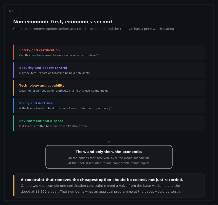
Safety and certification, security and export control, technology and capability, policy, environment and disposal. Transportability, where an item is too large or too fragile to be moved to a distant facility at all, is usually handled inside the technology and capability gate rather than as a sixth one. Each gate either removes an option at a level or it does not. Two rules keep this step honest: the reason is recorded against the item, and where a gate removes the option the economics would have chosen, the difference is computed and reported as the price of the constraint.
5. Build the cost model on capability, not on repairs
The quantity being compared is the annual cost of owning the capability, which is a different thing from the cost of a repair. Every option carries:
- Recurring: replacement buys or repair materials, labour, transport, calibration, holding cost of stock.
- One-off, annualised: test equipment per site, initial training per site, technical data per level, facilities, and the pipeline spares the option forces you to buy.
The pipeline term is the one most often left out, and it follows directly from the turnaround time: an item away being repaired has to be replaced on the equipment from stock, so the expected number in the pipe is demand × turnaround ÷ 365, plus a safety level for variability. A long depot round trip buys cheap labour with expensive stock.
Where the programme has an availability or a turnaround requirement, it enters here rather than at the end. There are two honest ways to impose it. Remove the options whose pipeline cannot return an item to the equipment inside the required time, which turns availability into another screening gate; or hold the requirement fixed, buy each option whatever stock it needs to meet it, and compare the options with that stock inside them. The second is the more useful and the more work, and it is what the published joint level-of-repair and spares formulations do properly. Neither is a substitute for saying, in the report, which one was used.
6. Work down the indentures
Decide the parent, then its children, then theirs. The parent's decision sets the place where each child's decision is taken and the shipping the child inherits, but it does not set the child's answer: a unit repaired at the depot will usually have most of its modules discarded there, and that is a normal result rather than an inconsistency.
Where the answers interact strongly, the honest treatment is to evaluate the combinations rather than the items one at a time. The published optimisation models do exactly that, and they exist because sequential item-by-item decisions can miss a cheaper joint answer, particularly when several items would share one tester.
7. Sweep the inputs that are soft
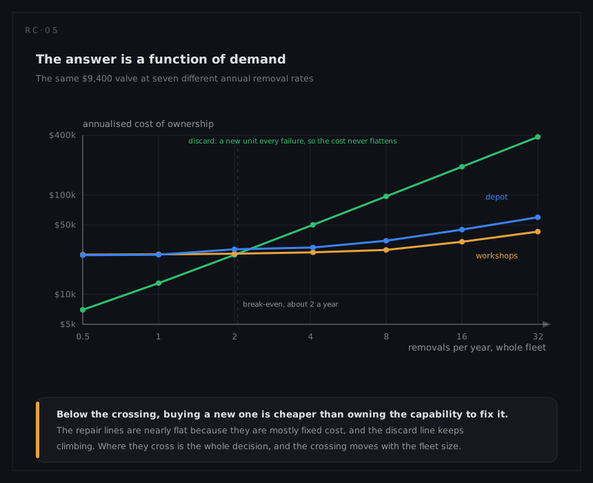
At minimum, sweep annual demand and unit price, and report the break-even for each. Two results deserve their own line in the report:
- Items near a boundary. A two per cent margin is not a decision. Say so, and recommend the option that is cheaper to change later.
- Items whose answer flips inside the credible range of the demand estimate. Those are the items where the field data will settle it, and the report should say what to watch.
8. Turn the decision into instructions
An answer that stays in the analysis changes nothing. It has to become:
| Output | Form |
|---|---|
| The repair level per item, and discard where that is the answer | The maintenance policy code carried on the item's logistics record |
| Support and test equipment | A procurement list, with quantities per site |
| Spares | The pipeline and stock the chosen option requires, at each site |
| Technical data | Which repair procedures are written, and to what depth |
| Training | Which trades, at which sites, for which items |
9. Redo it, on a trigger rather than on a calendar
Four things move the answer: fleet size, usage, prices and observed failure rates. When one of them moves far enough that an item crosses a break-even computed in step 7, the analysis is out of date whatever the date on it says. That is why the break-evens are worth carrying forward: they turn the next review from a repeat of the whole study into a check against four numbers.