

A maintainability prediction is an exercise in adding up small times and then dividing correctly. Both halves go wrong in characteristic ways.
The elemental activities
A corrective repair decomposes into a fixed set of activities, and estimating each separately is what makes the total arguable rather than asserted:
| Activity | What it covers |
|---|---|
| Localisation | Determining that something is wrong and roughly where |
| Isolation | Determining which replaceable item it is |
| Disassembly | Gaining access: covers, brackets, harnesses, adjacent items |
| Interchange | Removing the failed item and fitting the replacement |
| Reassembly | Putting back everything disassembly disturbed |
| Alignment | Adjustment, configuration, calibration after fitting |
| Checkout | Verifying the repair and returning the equipment to service |
Two of those are diagnosis and four are mechanical work. Which pair dominates is an empirical question per design, and the answer is usually the mechanical one, which is why maintainability is a packaging discipline as much as a diagnostic one.
The weighting, and why it is the whole method
The mean corrective maintenance time is not the average of the task times. It is the average a technician actually experiences, which weights each repair by how often it arrives:
Mct = Σ (λᵢ · tᵢ) ÷ Σ λᵢ
Every failure rate in that expression comes from the prediction, which is what keeps the two analyses consistent. The unweighted average of the same task times is a different and meaningless number, and it is the one a spreadsheet produces by default.
The same weighting gives the useful ranking. The product λᵢ tᵢ is the technician's time per item per unit of operating time, and sorting by it answers "where does the maintenance budget go" in a way that neither the failure-rate list nor the repair-time list can.
The distribution, and the percentile
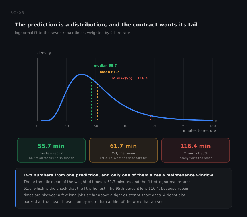
Repair times are skewed: a cluster of short jobs and a tail of long ones, because the things that make a repair long (access, alignment, a difficult diagnosis) multiply rather than add. The lognormal is the standard model, and it is fitted on the logarithms:
μ = Σ λᵢ ln tᵢ ÷ Σ λᵢ and σ² = Σ λᵢ (ln tᵢ − μ)² ÷ Σ λᵢ
from which the median is e^μ, the mean is e^(μ + σ²/2), and the percentile that contracts actually specify is
Mmax(p) = e^(μ + zp σ) with z = 1.282 at 90 per cent and 1.645 at 95
The mean and the percentile are far apart and both are needed. In the worked example the mean is 61.7 minutes and the 95th percentile is 116.4, nearly double it: a depot slot booked at the mean is overrun by more than a third of the work that arrives.
A useful internal check falls out of the two ways of computing the mean. The weighted arithmetic mean of the task times and the fitted lognormal's e^(μ + σ²/2) should agree closely; where they do not, the lognormal is a poor description of that particular mix, which usually means two populations have been averaged into one.
The five procedures of MIL-HDBK-472
The handbook does not contain one method. It contains five: four in the 1966 base document and Procedure V added by Notice 1 in 1984. They differ in what they need and what they return, so naming the procedure is part of stating the result.
| Procedure | What it needs | How it works | Where it fits |
|---|---|---|---|
| I | Elemental activity times, and the time structure of a fix | Synthesises the distribution of downtime from those elemental times, by Monte Carlo sampling | Airborne electronics, on the flight line |
| II | A parts list, a maintenance concept and task times per part class | Builds the equipment's corrective and preventive times from the task times of its part classes | The final design stage; all systems and equipments, though non-electronic task times have to be estimated |
| III | A random sample of maintenance tasks, and a design to score | Scores each sampled task against design checklists and converts the scores to a time through a regression equation | Ground electronics |
| IV | A comparable predecessor, or people who have maintained one | Task times from historical experience and expert judgement | All systems and equipments; it leans on experience rather than on design detail |
| V | A defined maintenance concept and an item list | Task-by-task synthesis from elemental activity times, Method A for early design and Method B for detailed | Avionics, ground and shipboard electronics, at organisational, intermediate and depot level: the one this module works through |
Procedure V is the one to know, and its two methods differ in where the elemental times come from. Method A scores them against checklists of design attributes while the design is still fluid; Method B takes them from the task as actually defined, on a design detailed enough to walk through. Both produce the same output: a time per repair, weighted into a mean and fitted for a percentile.
Two rules travel with the choice. One procedure per prediction, because two procedures produce numbers with different meanings and adding them produces neither. And the procedure is named in the report, because a reader who does not know which one was used cannot tell whether the figure is a checklist score, an experience estimate or a task-by-task synthesis.
Maintenance levels, and why the same failure has three answers
A repair happens somewhere, and where it happens decides what the task is. The conventional split is three levels, and a prediction is made per level rather than once:
| Level | Where | What a task is | What the number is used for |
|---|---|---|---|
| Organisational | On the equipment, in service | Remove and replace the failed assembly | Availability, and the operator's downtime |
| Intermediate | A workshop or depot road | Repair the assembly by replacing the failed item inside it | Workshop manning, turnaround, spares float |
| Depot | A specialist facility or the manufacturer | Repair the item itself, to component level | Repair cost, scrap policy, level-of-repair decisions |
The same cabinet gives three different numbers:
| Level | Task | Time |
|---|---|---|
| Organisational | Swap the whole converter | 55 min |
| Intermediate | Swap the failed item inside it | 62 min |
| Depot | Repair the failed card | 210 min |
Availability uses the time for whichever action returns the equipment to service. Under the usual concept, repair by exchange, that is the organisational number: the workshop's 62 minutes happens afterwards and in parallel with the equipment running, so quoting the intermediate figure into an availability model is a common and expensive error and quoting the depot figure into one is worse. Where the concept is repair in place, with the equipment out of service while the item inside it is changed, the restoring action is that in-place repair and its time is the one the availability model wants. The test is not the label on the level; it is which task the equipment is waiting on.
Which level a programme is even allowed to do the work at is a level of repair analysis decision, and it is settled before this prediction can be made.
The measures, and which one answers which question
A maintainability prediction produces a family of quantities, not a single MTTR, and each answers a different question:
| Symbol | Name | Expression | Answers |
|---|---|---|---|
Mct | Mean corrective maintenance time | Σ λᵢ tᵢ ÷ Σ λᵢ | How long a repair takes, on average |
Mpt | Mean preventive maintenance time | Σ fⱼ tⱼ ÷ Σ fⱼ over scheduled tasks | How long a scheduled task takes |
M̄ | Mean active maintenance time | (λ·Mct + f·Mpt) ÷ (λ + f) | How long any maintenance action takes |
Mmax(p) | Maximum corrective time at a percentile | e^(μ + zp σ) on the log times | How long a slot has to be |
MMH/OH | Maintenance man-hours per operating hour | Σ λᵢ tᵢ cᵢ + Σ fⱼ tⱼ cⱼ, corrective and preventive, with crew size c | How many people the fleet needs |
MDT | Mean down time | M̄ plus logistic and administrative delay | What the operator actually loses |
MMH/OH is the one a support contract is usually priced on and the one this analysis is least often used to produce. It differs from Mct in two ways that both matter: it counts crew size, so a two-person lift costs twice its clock time, and it counts preventive work, the second sum in that expression, which Mct excludes entirely and which on most equipment is the larger number.
One note on the symbols, because the literature writes them differently. A mean is conventionally marked with an overbar, so what the handbooks print as M̄ct and M̄pt are the quantities written Mct and Mpt here and on the maintainability page: one convention across this knowledgebase, with the overbar kept only for M̄ itself, the mean active maintenance time, which carries no subscript. Mmax is a percentile rather than a mean and never took an overbar in either form.
What the numbers are worth
An elemental time is a judgement about how long a trained person takes to undo six fasteners, on hardware that does not exist, in a posture nobody has tried. Three consequences follow, and the honest presentation states all three:
- Absolute accuracy is modest. A factor of two on any individual task time is unremarkable.
- Comparative accuracy is good. Two arrangements estimated by the same person with the same library rank correctly far more often than either estimate is right.
- The ranking is robust. The contribution list survives large errors in individual times, because it is dominated by the product of two quantities that are both large.