

Testability's mathematics is bookkeeping over the failure-mode inventory: which modes each test sees, to what group of suspects each symptom points, and how often the tests speak when nothing is wrong. The quantities are simple ratios; the craft is in the weighting, the denominators, and the honesty of the underlying mode list. This chapter builds the measures, maps them onto the functional-safety vocabulary of dangerous detected and undetected failures, shows why failure-rate weighting changes everything, lays out the test layers that generate the coverage, prices ambiguity, and ends with the dependency matrix that computes it all before hardware exists, worked line by line.
Notation used in this topic
| Symbol | Reads as | Meaning |
|---|---|---|
| FDR | fault detection rate | rate-weighted detection coverage |
| FIR | fault isolation rate | of detected failures, the share resolved to at most n units |
| 1 − FDR | undetected fraction | the failures nothing announces; feeds the latent ledger |
| BIT | built-in test | test capability designed into the item itself |
| CBIT, PBIT, IBIT | continuous, power-up, initiated BIT | the three in-service test layers |
| CND, RTOK, NFF | cannot duplicate, retest OK, no fault found | the field honesty measures |
| λ | lambda | failure rate; every coverage figure is weighted by it |
λS, λD | safe and dangerous failure rate | the functional-safety split of λ by effect on the safety function |
λDD, λDU | dangerous detected, dangerous undetected | the split of λD by whether a diagnostic finds it, in time |
| DC | diagnostic coverage | λDD / λD: coverage over the dangerous population only, and not FDR |
| SFF | safe failure fraction | 1 − λDU / λ: an architectural gate, not a diagnostic measure |
| T | proof-test interval | the period between exercises of a dormant item |
Tdiag | diagnostic test interval | how often an automatic diagnostic runs, distinct from T |
| λT/2 | the average latent unavailability of a dormant item between tests, valid only while λT ≪ 1 | |
FARh, FARr | false alarm rate, false alarm ratio | per operating hour, and as a share of all annunciations |
One naming note, because the literature is split. The older diagnostics standards call these quantities the fraction of faults detected and the fraction of faults isolated, abbreviated FFD and FFI. They are the same two ratios under different names, and this book uses FDR and FIR throughout because that is what appears in specifications, in contracts and alongside FAR, which has no FF-form at all.
Every abbreviation used anywhere in RAMS Core is defined in the glossary.
The coverage measures
| Measure | Definition | The trap |
|---|---|---|
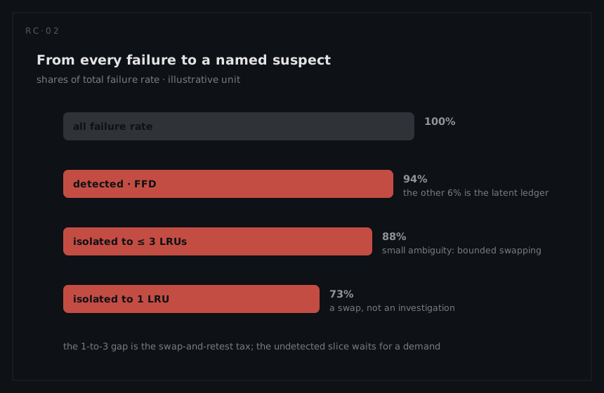
| Fault detection rate (FDR) | The failure-rate-weighted fraction of failures detected by the stated test means | Quoted mode-counted, or against a censored mode list, it flatters |
| Fault isolation rate (FIR to n) | Of detected failures, the fraction isolated to an ambiguity group of ≤ n replaceable units | FIR to 1 and FIR to 3 are different worlds for the technician |
False alarm rate, FARh | Indications of failure when none exists, per operating hour | The maintenance load: it multiplies by fleet hours into removals |
False alarm ratio, FARr | The same indications as a share of all annunciations, FARr = false / (true + false) | The credibility budget: it decides whether the crew believes the next caption |
| Cannot duplicate (CND) | Field indications that maintenance cannot reproduce | The false-alarm rate as the field actually experiences it |
| Retest OK (RTOK) | Removed units that test good at the next level | The isolation shortfall as the supply chain experiences it |
| Undetected fraction (1 − FDR) | The failures nothing announces | The latent ledger: its dangerous part is the λDU that availability's λT/2 arithmetic runs on |
Every number in the table is conditional on three declarations that belong in the same sentence as the value: which test means (continuous monitors only? plus initiated tests? plus shop equipment?), which failure universe (the full FMEA mode list, weighted by rate), and which replaceable-unit level (isolation to an LRU at the flight line is not isolation to a card in the shop). A coverage claim without its conditions is unfalsifiable, exactly as a reliability claim without a mission profile is.
Coverage in functional-safety vocabulary
The measures above come from the diagnostics lineage: one failure population, one detected share, one denominator. Functional safety asks the same physical question and partitions the population differently, because it cares about exactly one consequence class. An engineer arriving from IEC 61508 or one of its sector applications (IEC 61511 in process, EN 50129 in rail, ISO 26262 in automotive, and the machinery sector's own derivatives) will be asked for coverage in that partition and will find none of these names in it. The two vocabularies describe the same monitors and are not interchangeable arithmetic.
The two cuts
The first cut splits the failure rate by what the failure does to the safety function:
λ = λS + λD
The second splits the dangerous half by whether an automatic diagnostic finds it:
λD = λDD + λDU
| Symbol | Reads as | The population it names |
|---|---|---|
λS | safe failure rate | failures that drive the item to the safe state, or leave the safety function still able to act |
λD | dangerous failure rate | failures that defeat the safety function, or would if a demand arrived |
λDD | dangerous detected | the dangerous failures an automatic diagnostic finds, and finds soon enough to matter |
λDU | dangerous undetected | the dangerous failures nothing finds until a proof test or a real demand |
Two properties of the cut deserve stating, because both are judgments made mode by mode in the FMEA rather than facts read off a datasheet. The classification is by effect on the safety function, not by severity of the item's own failure: a power supply that fails hard and trips the plant is a safe failure, while a sensor stuck mid-range while the process runs away is a dangerous one. And modes with no effect on the safety function at all are treated separately, sometimes excluded from the calculation entirely, which is one of the standard places two competent analyses of the same item stop agreeing.
Diagnostic coverage is not FDR
DC = λDD / λD
This is the coverage quantity IEC 61508 actually credits, and it is a different ratio from FDR. FDR is weighted over the whole failure population; DC is weighted over the dangerous population only. When the detections being credited are the dangerous ones, the two share a numerator and differ in denominator, so their ratio is fixed by the split alone:
DC / FDR = λ / λD
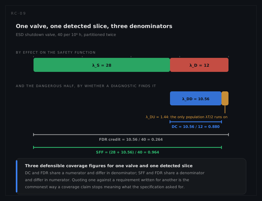
The compressor train's shutdown valve puts numbers on the gap. The compressor page gives the valve 40 per 10⁶ hours in total, of which 12 is dangerous and, before any partial stroke is credited, dangerous with nothing watching it: λS = 40 − 12 = 28 and λD = λDU = 12 per 10⁶ hours. The quarterly partial stroke is credited with 88% of that dangerous population, which converts it:
λDD = 0.88 × 12 = 10.56 per 10⁶ h λDU = 12 − 10.56 = 1.44 per 10⁶ h
DC = λDD / λD = 10.56 / 12 = 0.880 FDR credit of the same test = λDD / λ = 10.56 / 40 = 0.264
One test, one valve, one set of detected failures, and two defensible coverage figures a factor of 40/12 = 3.3 apart. Quote the 88% against a requirement written for FDR and the valve's detection is overstated threefold; quote the 26.4% into a safety integrity calculation and an adequate diagnostic is discarded and replaced with hardware nobody needed. Neither figure is wrong and neither is a conversion of the other. The denominator is the entire content of the disagreement, which is why it belongs in the same sentence as the value, exactly as the three declarations in the previous section do.
Safe failure fraction
SFF = (λS + λDD) / (λS + λD) = 1 − λDU / λ
The second form is the one to carry: SFF and FDR share a denominator and differ in numerator, precisely as DC and FDR share a numerator and differ in denominator. For the valve, before the partial stroke SFF = 1 − 12/40 = 0.700, and with it credited SFF = (28 + 10.56)/40 = 0.964.
SFF is not a diagnostic measure, and reading it as one is the mistake it invites. Under IEC 61508-2 Route 1H it caps the claimable integrity level for a given hardware fault tolerance and element type: the valve, a Type A element with no fault tolerance, is held to SIL 2 at 70 per cent and would need 90 per cent before SIL 3 could be claimed. Route 2H and IEC 61511's field-device tables reach the same architectural constraint without computing SFF at all. The point of the constraint is that a strong probability-of-failure-on-demand number cannot be claimed on a single non-redundant channel that diagnoses nothing about itself. The formula also displays its own weakness. Hold λDU fixed and SFF rises as λ grows, so acquiring safe failure modes improves the fraction while changing nothing dangerous: the same valve with twice the total rate, every added failure safe, would score 1 − 1.44/80 = 0.982 and carry an identical probability of failure on demand. Safe failures are not good news, they are lost production, and an SFF improved by collecting them has improved nothing the safety case rests on.
The diagnostic interval and the process safety time
λDD is not a property of a monitor. It is a property of the monitor, the interval at which it runs, and the reaction that follows it, and functional safety enforces that with two clocks. The diagnostic test interval Tdiag is how often the diagnostic actually executes: milliseconds for a processor watchdog, three months for the valve's partial stroke. The process safety time is how long the equipment under control takes to reach the hazardous condition after the failure, with the safety function absent. For functions in high-demand or continuous mode, IEC 61508-2 requires the diagnostic test interval plus the time to achieve the safe state to be less than the process safety time.
A diagnostic that misses that deadline has detected nothing the arithmetic can use, and its share of the dangerous population stays in λDU however complete its coverage looks on paper. Detection is a claim about timing, not about visibility, and an entry that lands in a log after the event is evidence for the investigation rather than credit in the safety case. The same structure appears in the availability ledger as detection latency: on the storage array one hour of monitor latency spends 30% of a five-nines annual budget without a single failure going undetected. Different currency, identical argument.
Low-demand functions run the clock differently, because no continuous monitor is racing a process. There, a diagnostic executing far more often than the proof test is credited as a reduction in λDU rather than as a shortening of T, which is exactly what the compressor page does with a quarterly partial stroke against an annual full stroke. The credit is legitimate only while C·Tdiag ≪ (1 − C)·T, and the full expression carries both exposures:
PFD ≈ λDU[(1 − C)·T/2 + C·Tdiag/2]
The compressor page quotes the first term alone, which is the convention the sector uses and is worth naming as one rather than mistaking for the whole.
What carries into the rest of this book
PFD ≈ λDU × T / 2
Every latent-exposure calculation in RAMS Core runs on λDU and on nothing else: the sawtooth in the availability foundations, the proof-test intervals throughout the safety examples, and the compressor valve's residual 1.44 per 10⁶ hours after partial stroke. The undetected fraction 1 − FDR is not that population but a superset of it, because it carries the safe undetected failures too, and putting it into λT/2 overstates the risk in the same way that putting the item's total rate in does. The safety page makes the same point from the other side.
Functional safety offers no counterpart to FIR. It never asks which unit to replace, only whether the function will act, so the isolation half of testability sits outside the standards entirely and is priced in the maintenance ledger instead. ISO 26262 partitions the population differently again, into a single-point fault metric and a latent-fault metric alongside a probabilistic metric for random hardware failures, with diagnostic coverage sitting inside both. The habit that transfers across all of them is one line long: read the denominator before quoting the number.
Coverage is failure-rate-weighted
The single most consequential convention in testability arithmetic: coverage is weighted by failure rate, not counted by mode. The definition of detection coverage is
FDR = Σλ(detected modes) / Σλ(all modes)
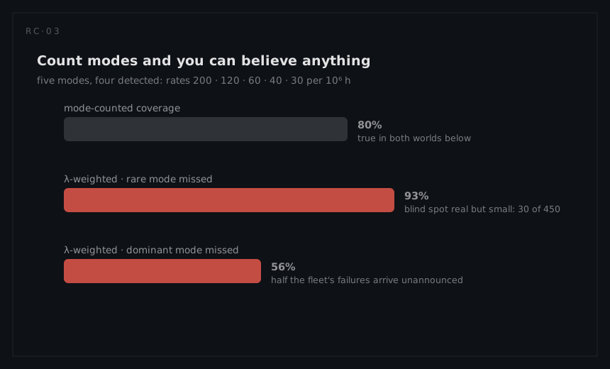
because the fleet does not experience modes with equal probability; it experiences them in proportion to their rates. A worked pair on an invented five-mode unit makes the point brutally. Let the modes carry rates 200, 120, 60, 40, 30 per 10⁶ hours (Σλ = 450), with four of the five detected. Mode-counted coverage is 80% in both of the following worlds. If the undetected mode is the 30 (the rarest mechanism in the list), weighted coverage is 420/450 = 93.3%: the blind spot is real but small. If the undetected mode is the 200 (the dominant mechanism), weighted coverage is 250/450 = 55.6%: nearly half the failures the fleet will actually have arrive unannounced, behind a proudly quoted "80% of failure modes covered". The weighting rule has two immediate corollaries: the failure-rate prediction is a load-bearing input to every testability number, and the highest-rate modes deserve detection design attention out of all proportion to their count.
The test layers
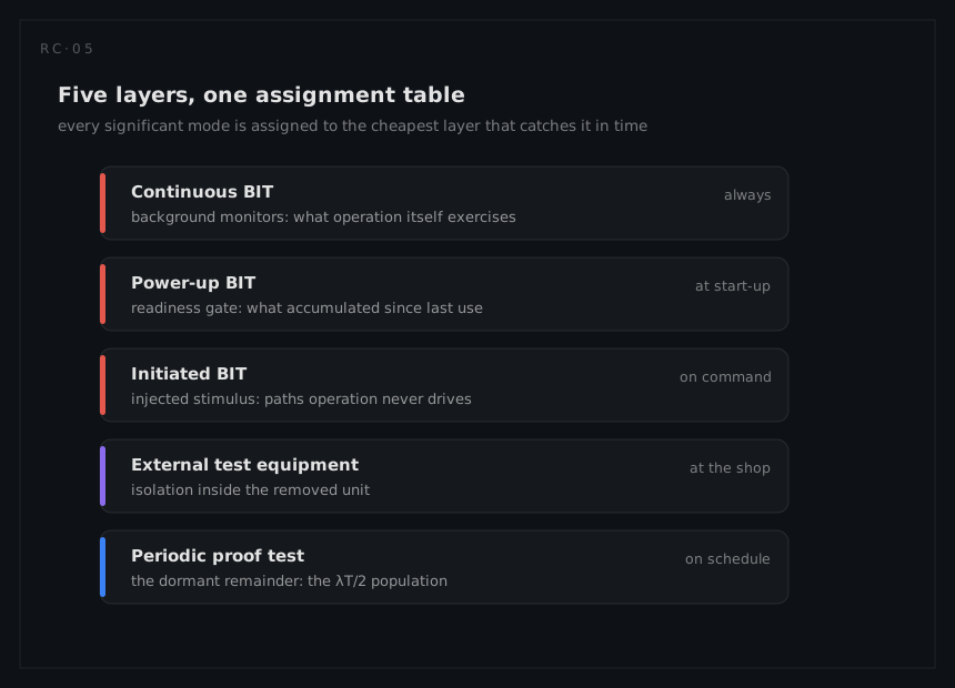
Coverage is generated by a stack of test means, each with its own trigger, reach, and cost, and a coverage claim is meaningless until it names its layers:
| Layer | When it runs | What it catches | What it costs |
|---|---|---|---|
| Continuous BIT (CBIT) | Always, in the background | Failures with observable signatures in normal operation | Sensors, processing margin, and the false-alarm exposure of always-listening |
| Power-up BIT (PBIT) | At start-up | Failures accumulated since last use; readiness gating | Start-up time; only as fresh as the last power cycle |
| Initiated BIT (IBIT) | On command, with stimulus | Failures needing injected test signals; deeper paths CBIT cannot exercise | Function interruption; operator or maintainer action |
| External test equipment | At the shop or depot | Isolation inside the removed unit; the SRU-level verdict | The test-programme development and the pipeline it lives in |
| Periodic proof test | On the maintenance schedule | Dormant functions nothing else exercises | The test-interval economics of the latent ledger |
The layers trade against each other by design. What CBIT does not watch, PBIT may catch a mission too late; what no BIT can stimulate waits for IBIT or the shop; and the dormant fraction that only a proof test exercises is precisely the population whose unavailability grows as λT/2 between tests. A testability architecture is the deliberate assignment of every significant failure mode to the cheapest layer that catches it soon enough for that mode's consequences, and the assignment table (mode by mode, from the FMEA) is the design artefact everything else audits against.
Ambiguity and its price
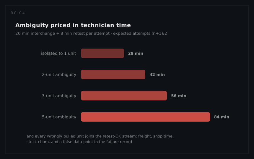
Isolation coverage is stated against ambiguity groups: the set of replaceable units a symptom cannot distinguish between. Requirements follow a standard pattern (a large fraction isolated to a single unit, nearly all to a small group, the remainder conceded to manual troubleshooting), and the group size converts to time and money mechanically. With equal priors over a group of n, sequential swap-and-retest resolves the fault after (n+1)/2 attempts on average: a 20-minute interchange inside a three-unit group becomes 40 minutes of expected swapping plus the extra verification cycles, before counting the deeper cost: every wrongly pulled unit enters the retest-OK pipeline, consuming transport, shop time, and stock, and depositing a false data point in the failure records. The maintainability systems chapter carries the same arithmetic from the repair-time side; here the point is attribution: ambiguity is not a maintenance problem, it is a design output, fixed by partitioning and test placement decisions, and no amount of technician skill can isolate what the design made indistinguishable.
False alarms and the no-fault-found family
The measures that decide whether a testability design survives contact with the field are the honesty measures. A false alarm is the test speaking when nothing is wrong; in the field it matures into a cannot duplicate (the crew saw the indication; maintenance cannot reproduce it) or, one step later, a retest OK (the removed unit tests good at the next echelon). The three form one pipeline, and its economics are vicious: each event consumes a full diagnostic and often a removal, and the stream's real product is erosion of trust. A crew that has been burned learns to ignore the annunciation, at which point the detection coverage so carefully engineered is worth exactly nothing; the boy-who-cried-wolf failure mode is the terminal state of dishonest BIT.
The engineering countermeasures are threshold and time discipline: persistence filters (an indication must survive n samples before latching), condition gating (suppress monitors in regimes where they are known to trip falsely), voting across redundant sensors, and richer signatures over single thresholds. Each filter trades a sliver of detection latency against false-alarm mass, and the trade must be designed, not defaulted, because the intermittent failure that a persistence filter smooths away is often the very fault the crew reported. The field data closes the judgment loop: CND and RTOK rates per unit, tracked through FRACAS, are the measured truth of the false-alarm budget, and a unit at the top of the RTOK Pareto is either a BIT threshold problem or an ambiguity problem wearing maintenance's uniform.
How coverage is computed: dependency modelling
Before hardware exists, every number above comes from a model with a stubbornly simple shape: a dependency matrix between failure modes and tests. Each row is a failure mode from the FMEA, carrying its rate from the prediction; each column is a test or monitor; each cell records whether that test responds to that mode. From this matrix the whole measure family falls out mechanically: detection coverage is the rate-weighted share of rows with at least one responding test among the claimed layers; isolation follows from the response signatures (two modes with identical signatures are indistinguishable, and the set of units hosting them is the ambiguity group); and the marginal value of any proposed test point is computable as the signatures it splits.
The smallest matrix that shows the whole machine
Take the invented five-mode unit from the weighting section, with its rates of 200, 120, 60, 40 and 30 per 10⁶ hours, and give the modes a home: module A carries the input and supply stage, and modules B and C sit in series in the signal path downstream of it. Three tests exist. A continuous rail monitor watches A's supply. A continuous output check watches the unit's output, which is corrupted by anything wrong in B or in C. An initiated wrap test loops a stimulus out through B and C together and back, so it too responds to both. A one means the test responds to the mode; a zero means it does not.
| Failure mode | λ per 10⁶ h | Module | Rail monitor | Output check | Wrap test |
|---|---|---|---|---|---|
| M1 | 200 | A | 1 | 0 | 0 |
| M2 | 120 | A | 1 | 0 | 0 |
| M3 | 60 | B | 0 | 1 | 1 |
| M4 | 40 | C | 0 | 1 | 1 |
| M5 | 30 | B | 0 | 0 | 0 |
| Total | 450 |
Which modes are detected is the first reading, and it is a row test: a mode is detected if its row contains at least one one. M1 to M4 qualify. M5's row is all zeros, which is what an undetected mode looks like inside a dependency model, here a dormant mechanism in B that changes nothing any of the three tests observe until a demand arrives.
Σλ(detected) = 200 + 120 + 60 + 40 = 420 per 10⁶ h FDR = 420 / 450 = 0.933
the same 93.3% the weighting section reached, because this matrix is that section's first scenario: the blind mode is the rarest one. The undetected fraction is 30 / 450 = 0.067.
The signature of a mode is its row, read as an ordered response pattern. M1 and M2 both signal (1, 0, 0). M3 and M4 both signal (0, 1, 1). M5 signals (0, 0, 0). The signature is the complete list of everything the test set can say about a mode, so two modes carrying the same signature are indistinguishable by these tests, and no diagnostic procedure, however well written, separates them.
Identical rows are where ambiguity lives, and only some of them cost anything. Two pairs match here and only one is an ambiguity group. M1 and M2 share (1, 0, 0) but both live in module A, so the symptom still names one replaceable unit: at this level of repair that is two modes with one action, not ambiguity. M3 and M4 share (0, 1, 1) and live in different modules, so the same symptom names two suspects and nothing in the design distinguishes them. Ambiguity is therefore a property of the signature-to-unit mapping rather than of the signature itself, which is the arithmetic under the partitioning argument in the design chapter: these three tests would give perfect isolation if B and C were one replaceable module, FIR(1) = 1.000, and would lose single-unit isolation entirely if A were split in two, FIR(1) = 0.000, because M1 and M2 share a row. Not a single test changes in either case.
FIR is computed over the detected population only, because a fault nobody saw cannot be isolated. The detected 420 splits into 320 whose signature names one module and 100 in the two-module group:
FIR(1) = (200 + 120) / 420 = 320 / 420 = 0.762 FIR(≤2) = (320 + 100) / 420 = 420 / 420 = 1.000
and the group's price follows from the (n+1)/2 rule above, with n = 2:
E[removals per detected fault] = 0.762 × 1 + 0.238 × 1.5 = 0.762 + 0.357 = 1.119
so 0.119 / 1.119 = 10.6% of everything this unit sends for repair is serviceable, and in rate terms the group's 100 per 10⁶ hours of detected failures each carry half an extra swap: 100 × 0.5 = 50 per 10⁶ h of wrong removals, chargeable to one pair of identical rows.
One test point, priced exactly. Add a fourth test that genuinely reaches C alone, a wrap injected at the B-to-C boundary and closed at the unit output. Two rows change: M3 becomes (0, 1, 1, 0) and M4 becomes (0, 1, 1, 1), and every other row simply gains a zero. The signatures are now distinct, the ambiguity group is gone, and
FIR(1) = (200 + 120 + 60 + 40) / 420 = 420 / 420 = 1.000
while FDR stays at 0.933, because the new test responds only to a mode that was already detected. The whole value of that test point is 23.8% of the detected population moving from a two-module group to a named module, worth the 50 wrong removals per 10⁶ hours and nothing whatever in coverage. Now compare the alternative purchase. A test reaching M5 and nothing else takes FDR from 0.933 to 1.000, leaves M3 and M4 still sharing a row, and moves FIR(1) only to 350 / 450 = 0.778, a rise that comes from a newly detected and uniquely isolable mode joining the numerator rather than from any ambiguity being resolved. That second effect is a trap in its own right: FIR's denominator is the detected population, so every change in detection moves FIR even when no isolation has improved, and a before-and-after comparison that changed both is uninterpretable. A test point that splits a signature and a test point that reaches a blind mode buy different measures, and the matrix is the only thing that tells them apart before the money is spent.
The discipline the matrix depends on
The modelling discipline matters more than the algebra. The mode list must be the honest FMEA inventory, not the subset the BIT designer remembered; the dependency entries must reflect real signal reach (a monitor two connectors away from the mode may see nothing at the flight line); and the claimed layers must match the operational scenario being quoted. Run honestly, the dependency model is the testability twin of the reliability prediction: a design-stage forecast, auditable line by line, of numbers the field will eventually measure: FDR against the announced-failure share, FIR against the first-swap success rate, and the false-alarm budget against the CND/RTOK Pareto. The method topic walks the analysis itself; the point here is that testability is computable early, while the test points are still cheap.