

Six hundred volumetric infusion pumps in one hospital, each running about 2,500 hours a year, and one biomedical engineering department to repair them. A pump takes 45 minutes to fix. A pump that has failed is unavailable to the wards for twelve hours, and if the hospital had not bought forty spare pumps it would be thirty-nine.
Nothing about that sentence can be derived from a failure rate and a repair time. The availability of this fleet is decided by a queue: by how work arrives, how it batches, and how close the single repair channel runs to its own capacity. Queues near saturation are violently non-linear, which is why the standard availability formula is off by a factor of fifty here, and why this is the page in the column where simulation is not a luxury.
The technique, and why this one
A discrete-event Monte Carlo simulation of the fleet, its single repair channel and its loaner pool, with an M/M/1 queueing formula used as the closed-form sanity check. Three properties of the system rule out anything simpler. There are 600 items and one repair channel, so the dedicated-repair assumption behind every product rule in the composition chapter is false. The failure population is a mixture with genuinely different shapes in it, so an aggregate rate misleads about when work arrives. And the intervention under evaluation, a pool of loan units, does not change any failure rate or any repair time: it changes the coupling between the ward's demand and the bench's queue, which is a structure only a simulation can represent.
| Item | Availability model | Parameters |
|---|---|---|
| Pumping mechanism | Weibull (β = 1.6, η = 3,700 operating h) | λ = 300 per 10⁶ h, the fit's average rate |
| Occlusion sensor | exponential | λ = 150 per 10⁶ h |
| Air-in-line detector | exponential | λ = 120 per 10⁶ h |
| Dose controller board | exponential | λ = 90 per 10⁶ h |
| Battery | Weibull (β = 3.4, η = 5,300 calendar h), replaced at seven months | λ = 800 per 10⁶ h, two handling events a pump-year |
| Repair channel | single server queue, simulated | active repair 0.75 h; annual preventive service 0.5 h per pump |
| Loaner pool | inventory buffer, simulated | 40 pumps |
What the fleet actually experiences
The pump's aggregate rate is 1,460 per 10⁶ hours, so
failures per pump-year = 1,460 × 10⁻⁶ × 2,500 = 3.65
fleet arrivals = 3.65 × 600 = 2,190 a year
Fleet availability is 0.982 with the 40-pump loaner pool and 0.943 without it. Work backwards from each to the downtime it implies, because that is where the lesson is:
with pool: 0.018 × 2,500 = 45 hours per pump-year → 45 / 3.65 = 12.3 h per event
without pool: 0.057 × 2,500 = 142.5 hours per pump-year → 142.5 / 3.65 = 39.0 h per event
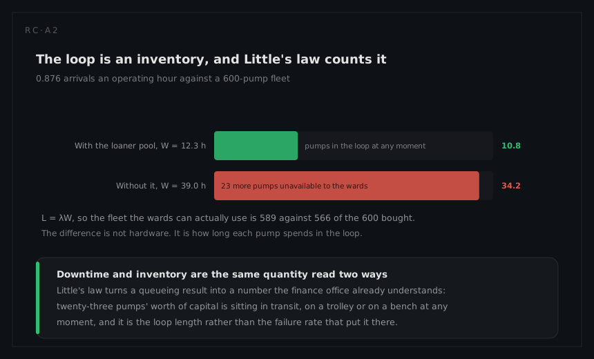
The active repair is 45 minutes in both cases. Between 94% and 98% of a pump's downtime is queue and turnaround, not work, and the technician's speed at the bench is close to irrelevant to the number the wards experience. Little's law confirms the same picture as an inventory count: at 0.876 arrivals per operating hour (2,190 over 2,500 hours), a 12.3-hour loop ties up 10.8 pumps at any moment and a 39.0-hour loop ties up 34.2, which is exactly the 589 against 566 usable pumps the two availability figures describe.
The queue, and why four points of utilisation matter
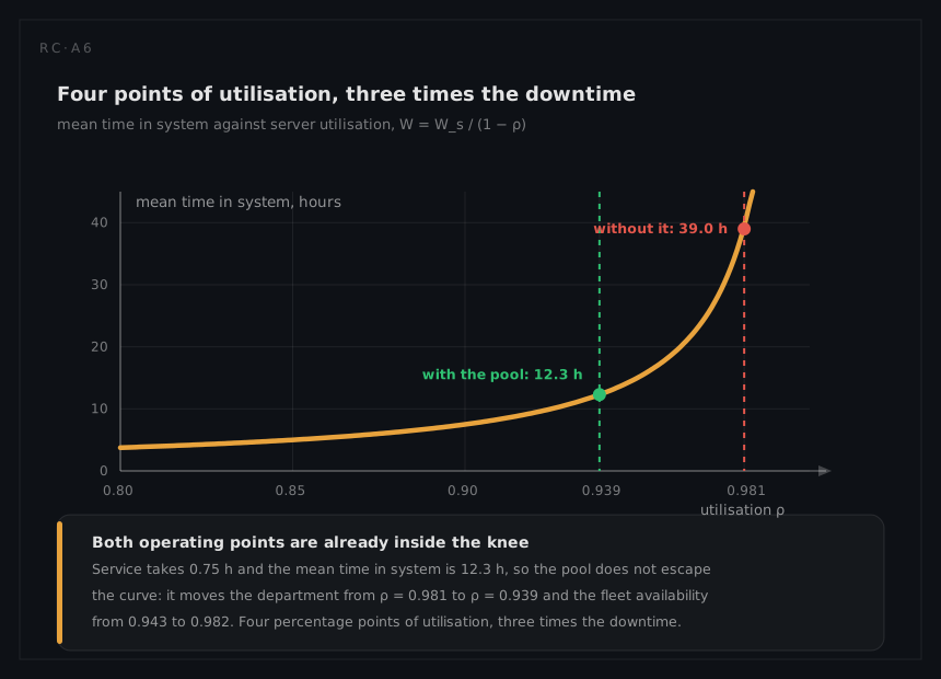
For a single-server queue the mean time in the system relates to the service time through the utilisation ρ:
W = Ws / (1 − ρ)
Substituting the two observed regimes with a service time of 0.75 hours:
with pool: 1 − ρ = 0.75 / 12.3 = 0.061 → ρ = 0.939
without pool: 1 − ρ = 0.75 / 39.0 = 0.019 → ρ = 0.981
Read that ρ for what it is: an effective utilisation of the whole ward-to-ward loop, not of the bench. The single server in this model is the entire collection, decontamination, queue, repair and return chain, and the 45 minutes is the work that chain is organised around rather than its only content. The maintainability page models the bench itself, two technicians and 3,000 productive hours a year against the 2,640 units that actually arrive there once the 450 no-fault-found returns are counted, and gets ρ = 0.733 with queueing and service together making up 8 per cent of the loop. The two numbers describe different servers and neither contradicts the other; quoting either as the technicians' workload is the mistake.
Four percentage points of utilisation, three times the downtime. That is the entire behaviour of a queue near saturation, and it explains two things that puzzle hospital finance departments. It explains why adding technician hours produces disappointing results at 94% utilisation and dramatic ones at 98%, since the gain is non-linear in the wrong direction for planning. And it explains why the pool works: without a buffer every arrival is an emergency that pre-empts whatever is on the bench, and pre-emption plus setup destroys throughput, pushing effective utilisation up precisely when demand is highest.
The staffing arithmetic completes the picture and rules out the obvious explanation:
corrective work = 2,190 × 0.75 = 1,642 hours a year
preventive work = 600 × 0.5 = 300 hours a year
total demand = 1,942 hours a year
which is roughly one full-time technician's worth of work. The queue that produces a twelve-hour mean downtime is therefore not caused by a gross shortage of labour: the implied loop capacity behind an effective ρ = 0.939 is about 2,069 hours a year, only 6% above the load. Availability problems built out of variability are solved with buffers, not with averages, and the loaner pool is the buffer.
Why the pool is not a spares pool
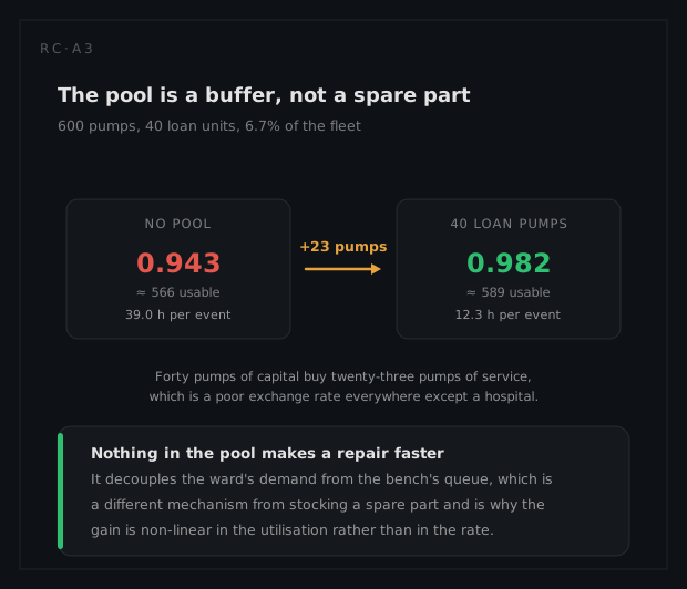
Nothing in the pool makes a repair faster. It means the ward's demand is met by a different physical unit while the failed one waits its turn, which is a different mechanism from stocking a spare part and produces a different kind of gain. Forty pumps, 6.7% of the fleet, move availability from 0.943 to 0.982: from about 566 to about 589 usable pumps. Buying roughly 23 pumps' worth of service for 40 pumps of capital looks like a poor exchange rate on paper and is an excellent one in a hospital, where the alternative to an available pump is not a delay but a clinical workaround.
This is also where the simulation earns its cost over the queueing formula. M/M/1 assumes Poisson arrivals, exponential service and no pre-emption, and none of those survives contact with a biomedical department that works shifts, batches similar repairs, and drops everything when theatre calls. The formula gets the shape of the answer right, which is why it is worth computing; the simulation gets the size right, and the size is what the capital request is written against.
The mixture hiding inside the arrival rate
The aggregate 1,460 per 10⁶ hours conceals a structure that decides the maintenance policy. The reliability page separates the population before fitting it, and the battery is the dominant term at 800 per 10⁶ hours, 55% of the pump's whole rate and therefore 55% of the queue's arrivals. Its fitted shape is β = 3.4, η = 5,300 calendar hours, and the replacement policy is a seven-month cycle, which is 5,300 hours: the characteristic life exactly. For any Weibull distribution the characteristic life is the 63.2% point, so
F(5,300) = 1 − exp(−(5,300 / 5,300)^3.4) = 1 − exp(−1) = 0.632
Nearly two thirds of batteries fail before their scheduled replacement, and therefore arrive at the bench as unplanned corrective work with a ward waiting behind them. Moving replacement to the B10 life inverts that:
B10 = η(−ln 0.9)^(1/β) = 5,300 × (0.10536)^(1/3.4) = 5,300 × 0.516 = 2,734 h
under four months, at which age nine batteries in ten are still healthy and the exchange is planned. That is not a reliability improvement; the battery is unchanged. It is an availability improvement obtained by moving arrivals from the queue that has a ward attached to it into a scheduled block that does not.
What the analysis tells the engineer to do
Change the battery at B10. Of the fleet's 2,190 maintenance actions a year, 1,750 arrive unscheduled, and the policy converts about 560 of those into planned exchanges. Because ρ is proportional to the unscheduled arrival rate when capacity is fixed, that takes utilisation from 0.939 to about 0.64 and mean downtime from
W = 0.75 / (1 − 0.64) = 2.1 hours
against 12.3. A sixfold reduction in what the ward experiences, from a maintenance-policy decision with no capital in it, and the queueing formula says so before anyone builds the simulation. The simulation's job is to check that the planned exchanges do not simply move the congestion into the service block.
Keep the pool, and size it against the simulation rather than against a rule of thumb, since the marginal pump is worth progressively less as ρ falls. And treat the 17% no-fault-found rate on returned pumps as an arrival-rate problem rather than a diagnostic curiosity: those returns are mostly setup error reported as device failure, they occupy the same single channel as real faults, and the testability page shows what the power-on self test can and cannot do about them. Every avoided false return is a slot in a queue running at 94% capacity.
What a different technique would have given
The alternative is the formula everyone reaches for: steady-state availability per pump.
MTBF = 10⁶ / 1,460 = 685 h
A = MTBF / (MTBF + MTTR) = 685 / (685 + 0.75) = 0.99891
Ninety-nine point nine per cent, against a fleet that actually runs between 94.3% and 98.2%. The formula is not wrong; it answers a question about one pump with its own dedicated technician standing next to it, and there are 600 pumps and one technician. It would also have made the loaner pool look absurd, because a fleet already at 0.99891 has nothing to buy, and the hospital would have spent the money on more reliable pumps and watched the wards' experience refuse to improve.
The second candidate, treating the fleet as a k-out-of-n parallel arrangement of 600 pumps against a demand for, say, 560, fails on the same assumption from the other direction. It would credit the redundancy while ignoring the shared repair channel, and redundancy served by one queue is not redundancy: it is 600 items taking turns in a single line.