

Two controller boards in active-active configuration, dual power supplies, drive shelves and a lithium backup unit protecting the write cache. The service target is five nines. Written as a percentage that is 0.99999, which conveys nothing; written as a budget it is 5.3 minutes a year, and once that number is on the page the interesting question is no longer how to achieve it but what could conceivably be allowed to spend it.
This is also the page in the column where the constant failure rate is genuinely correct and should be defended rather than apologised for. Screened parts, a controlled machine room, useful-life operation, and a service life shorter than the onset of any wear-out mechanism in the bill of materials: the exponential assumption is not a convenience here, it is a description.
The technique, and why this one
A Markov state model of the repairable controller pair, whose transitions are detection and dispatch rather than repair, expressed throughout as a downtime budget in minutes per year. The Markov model is required because the two controllers are served by one field-service contract, so the second failure during the first one's outage does not get its own independent repair channel, and the product rule's dedicated-repair assumption fails. Minutes rather than percentages are required because at five nines the significant digits live past the point where a percentage is readable, and because budgets in minutes add down a series chain and can therefore be allocated like any other budget.
| Item | Availability model | Parameters |
|---|---|---|
| Controller board (2 fitted) | exponential, Markov pair, shared service channel | 3,000 FIT = 3.0 per 10⁶ h each; 4-hour on-site response |
| Power supply (2 fitted) | exponential, hot-swappable | 1,500 FIT = 1.5 per 10⁶ h each |
| Lithium backup unit | exponential, state-of-health monitored | 900 FIT = 0.9 per 10⁶ h |
| Drives | renewal process, not a survival question | 0.4% annualised failure rate |
| Firmware update | scheduled event, not a distribution | 20 minutes if disruptive |
| Repair | absent by design | everything customer-replaceable is hot-swappable |
The nines, as a budget
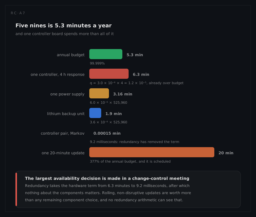
A year is 525,960 minutes, so the whole family of targets converts directly:
| Target | Unavailability | Downtime per year |
|---|---|---|
| 0.999 | 1 × 10⁻³ | 8.8 hours |
| 0.9999 | 1 × 10⁻⁴ | 52.6 minutes |
| 0.99999 | 1 × 10⁻⁵ | 5.3 minutes |
| 0.999999 | 1 × 10⁻⁶ | 31.6 seconds |
Each nine is a factor of ten, and the practical consequence is that the levers change character between rows rather than getting harder. Four nines is a hardware and repair problem. Five nines is a detection, dispatch and change-management problem, because at 5.3 minutes a year the mean time to notice a fault is a larger term than the mean time to fix it.
The single controller, and the term that is not repair
Unavailability of one controller is the familiar product of rate and downtime:
q = λ × MDT = 3.0 × 10⁻⁶ × 4 = 1.2 × 10⁻⁵
1.2 × 10⁻⁵ × 525,960 = 6.3 minutes a year
A single controller board, on its own, already exceeds the five-nines budget. What makes this system unusual is the composition of the four hours. It is not a repair duration: everything customer-replaceable in this array is hot-swappable, so active repair time never enters the availability arithmetic at all. The four hours is the on-site response commitment in the support contract, which is detection plus dispatch plus travel. The maintainability page can shave minutes off the physical swap and this number will not move by a digit, while a monitoring gap that delays detection by one hour costs 25% of the term outright. When a design removes repair from the equation, the telemetry and the contract become the only two levers left.
The pair, and where the product rule stops
The instinctive next step is the parallel product rule:
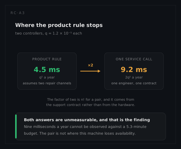
q² = (1.2 × 10⁻⁵)² = 1.4 × 10⁻¹⁰
1.4 × 10⁻¹⁰ × 525,960 = 4.5 milliseconds a year
That rule assumes each controller has its own repair channel. It does not: one engineer is dispatched, and while the first board is being replaced the second is unprotected with nobody available to attend it. The Markov solution for a two-unit repairable pair with a single repair channel carries a factor of two:
qpair = 2(λ/μ)² / (1 + 2λ/μ) ≈ 2 × (1.2 × 10⁻⁵)² = 2.9 × 10⁻¹⁰
2.9 × 10⁻¹⁰ × 525,960 = 9.2 milliseconds a year
Twice as bad, and still nine milliseconds. That is the instructive part. No storage array anywhere is down for nine milliseconds a year, so the model has plainly stopped describing the system: the shared backplane, the shared firmware build, the shared power feed and the shared operator all sit outside it, and between them they own effectively the entire 5.3-minute budget. A redundancy calculation that produces an absurd answer has not proved the design is perfect; it has proved that the remaining risk lives somewhere the model cannot see. The honest response is to stop refining the pair and go looking for the common terms, which is what fault tree analysis with an explicit common-cause treatment is for.
The ledger definition that moves a third of the budget
The lithium backup unit protects the write cache. At 900 FIT with the same four-hour response,
q = 0.9 × 10⁻⁶ × 4 = 3.6 × 10⁻⁶
3.6 × 10⁻⁶ × 525,960 = 1.9 minutes a year
which is 36% of the entire five-nines budget from one component. Or it is zero, depending on a definition. A failed backup unit does not stop the array; it forces the write cache into write-through mode, which is slower but functionally complete. If degraded performance counts as available, this line disappears; if it does not, it is the largest single hardware term on the page. One clause in the service-level agreement moves more than a third of the budget, which is more than any engineering decision available on this page. That is the partial-state ambiguity warned about in the foundations chapter, and it is why the definitions have to be published before the first report rather than negotiated after it.
The drives make the complementary point. At a 0.4% annualised failure rate, one drive fails per 250 drive-years, which across a populated array is a steady arrival rather than a rare event. The structure is designed to absorb it, so the availability question about drives is never whether one fails; it is whether a second fails inside the rebuild window opened by the first. The power supplies are the easy case: 1.5 × 10⁻⁶ × 4 = 6.0 × 10⁻⁶ each, a pair at 3.6 × 10⁻¹¹, hot-swappable, and not worth further attention.
The change window is the architecture
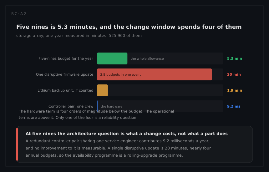
A single disruptive firmware update of 20 minutes costs
20 / 525,960 = 3.8 × 10⁻⁵
A = 1 − 3.8 × 10⁻⁵ = 0.999962
so one such evening a year caps the array at four nines regardless of how good the hardware is, and
20 / 5.3 = 3.8
nearly four years of the five-nines budget spent at once. Five nines on this array is a change-management property before it is a hardware property. Rolling, non-disruptive updates are not an operational convenience; they are the availability architecture, and a redundant pair that cannot be updated one side at a time is not redundant for availability purposes at all. The same logic runs through the shared firmware build noted above: two controllers running identical code are two controllers with one software failure mode, which is the reason the pair's 9.2 milliseconds is fiction.
What the analysis tells the engineer to do
Three actions, in budget order. Make every update rolling, because that single property is worth 3.8 years of budget and nothing else on this page comes close. Then attack detection, since the four-hour term is dominated by noticing and dispatching, and telemetry coverage at 97% is the number that decides how much of the failure rate ever reaches the clock at all; the 3% that does not is running latent, and a redundant pair with one silently failed side is a single string.
Then settle the write-through question in writing, before the first quarter's report. It is worth 1.9 minutes of a 5.3-minute budget, which makes it the largest hardware decision available, and it is made by a lawyer rather than an engineer unless an engineer insists on being in the room. Nothing on this list is a component improvement, and that is the finding: the pair sits at 2.9 × 10⁻¹⁰ against a 10⁻⁵ budget, four orders of magnitude clear of it.
What a different technique would have given
The plausible alternative is the pure reliability block diagram: series-parallel structure, independent repair, Q = Πqᵢ for the redundant pairs and Q = Σqᵢ for the chain. It would have given 1.4 × 10⁻¹⁰ for the controller pair instead of 2.9 × 10⁻¹⁰, understating it by half, which sounds serious and is not: the difference between 4.5 and 9.2 milliseconds a year is of no consequence whatever against a 5.3-minute budget.
The real reason it was rejected is that it would have declared the design finished. An RBD rolls up the hardware and reports an availability of essentially 1.0, which invites the programme to spend its remaining effort on component selection, derating and supplier quality: all of them useful, none of them capable of touching the two terms that actually consume the budget. The Markov model was not adopted because its number was materially better. It was adopted because building it forces the analyst to write down the repair channel, the detection interval and the shared resources explicitly, and the moment those are on the page it becomes impossible to keep pretending that the answer is 9.2 milliseconds.