

Two active-active controller boards, dual power supplies, populated drive shelves and a lithium backup unit protecting the write cache. Most of the other pages in this chapter have been arguments for moving away from the constant failure rate. This one is the argument for keeping it, because there is a class of system where the exponential model is not a convenience but the correct description, and knowing which class that is matters as much as knowing when to abandon it.
The technique, and why this one
Parts-count prediction in FIT, with a Markov model for the repairable pair and a renewal process for the drives. Constant λ is defended here rather than assumed, and the defence has four parts: the parts are screened and burned in, so the infant-mortality region has been removed before shipment; the operating environment is tightly controlled in temperature, humidity and power quality; the service life is deliberately shorter than the onset of any wear-out mechanism in the design; and the population is large enough that the aggregate arrival of failures is genuinely Poisson even where individual mechanisms are not.
| Item | Rate | Fitted | Model |
|---|---|---|---|
| Controller board | 3,000 FIT (3.0 per 10⁶ h) | 2, active-active | exponential, parts-count build-up |
| Power supply | 1,500 FIT | 2, hot-swappable | exponential |
| Drive | 0.4% annualised failure rate | many | renewal process |
| Lithium backup unit | 900 FIT | 1 | exponential rate, non-exponential consequence |
Where 3,000 FIT comes from
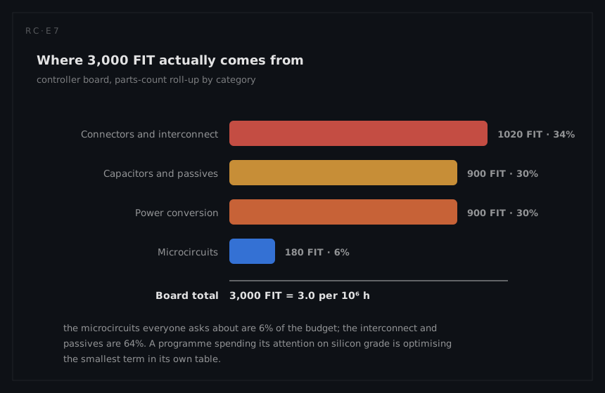
FIT is the local dialect: one FIT is one failure per 10⁹ device-hours, so 3,000 FIT is 3.0 failures per 10⁶ hours. The board's figure is not a guess; it is a parts-count roll-up over the bill of materials:
| Category | Contribution |
|---|---|
| Microcircuits | 180 FIT |
| Capacitors and passives | 900 FIT |
| Connectors and interconnect | 1,020 FIT |
| Power conversion | 900 FIT |
| Board total | 3,000 FIT |
The distribution of that total is the useful part. The microcircuits, the components everyone asks about, contribute 6% of the board's rate; the connectors and the passives contribute 64% between them. This is a general and repeatedly rediscovered result in electronics prediction: the failure budget lives in the interconnect and the passives, and a reliability programme that spends its attention on silicon grade is optimising the smallest term. The prediction topic works the underlying models.
What the constant rate predicts
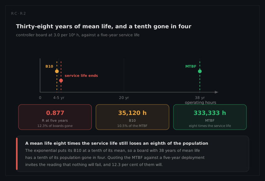
Fixing λ fixes everything else. For one board over a five-year service life of 43,800 hours:
MTBF = 1/λ = 1 / (3.0 × 10⁻⁶) = 333,333 h, or 38 years
R(43,800) = e^(−3.0 × 10⁻⁶ × 43,800) = e^(−0.1314) = 0.877
B10 = −ln(0.9)/λ = 0.10536 / (3.0 × 10⁻⁶) = 35,120 h, or 4.0 years
Thirty-eight years of mean life, 12.3% of boards failing within five years, a tenth of them gone by four. B10 is 10.5% of the MTBF for every exponential item whatever its rate, so an MTBF with no percentile beside it gets read as a life it does not describe.
The fixed hardware as a series chain, no redundancy credit:
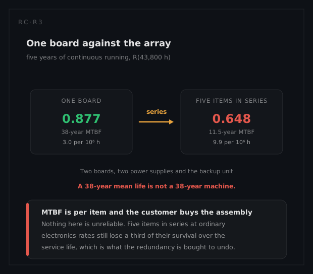
λseries = 2(3.0) + 2(1.5) + 0.9 = 9.9 per 10⁶ h, MTBF 101,010 h = 11.5 years
R(43,800) = 0.877 × 0.877 × 0.936 × 0.936 × 0.961 = 0.648
One array in three loses one of those five units inside five years. That 9.9 anchors two neighbours: the testability page divides it by 97% coverage and leaves 0.297 per 10⁶ h running silent, and the maintainability page turns the boards' 6.0 into 69 returned units a year per thousand arrays, 17 of them fault-free.
A second board with no repair at all gives 1 − (1 − 0.877)² = 0.985, turning a 12.3% five-year risk into 1.5%; everything more dramatic below is bought by repair rather than by redundancy. Confirming 3,000 FIT at 90% confidence with zero failures would need −ln(0.10)/λ = 767,500 board-hours, 87.6 years on one board or 384 hours across a thousand arrays.
Why the shape parameter stays at one
The exponential is the Weibull with β = 1, so the chapter's usual machinery runs here and returns nothing:
MTTF = η · Γ(1 + 1/β) = η · Γ(2) = 333,333 × 1 = 333,333 h
The gamma factor is exactly one and the characteristic life is the mean life. On the railway page the same expression at β = 1.9 gives Γ(1.526) = 0.8874 and 37,300 hours against an η of 42,000, and that separation is what makes preventive replacement at B10 = 13,000 hours worth planning. A barrier drive lifts a boom several hundred thousand times and the metal keeps count; a controller board in a temperature-controlled hall has no such counter running. Constant λ is a claim about where the service life sits on the bathtub curve, not a claim that nothing ages.
The repairable pair, and where the arithmetic stops being useful
A single controller with a four-hour on-site response has a steady-state unavailability of
q = λ/(λ + μ) ≈ λ·MDT = 3.0 × 10⁻⁶ × 4 = 1.2 × 10⁻⁵
That figure is this page's main export: 1.2 × 10⁻⁵ × 8,760 h = 0.105 h, 6.3 minutes a year against a five-nines budget of 5.3. One controller has overspent the year on its own, which is the reason there are two.
Two of them in parallel, but served by one field-service contract rather than two independent repair channels, solved as a three-state Markov chain, give a pair unavailability of approximately
qpair ≈ 2·(λ·MTTR)² = 2 × (1.2 × 10⁻⁵)² = 2.9 × 10⁻¹⁰
which corresponds to about nine milliseconds of downtime per year. Nobody believes that number, and nobody should. When redundancy arithmetic returns an absurdly good answer, the model has stopped describing the system. What will actually take this array down is not two independent board failures coinciding: it is the shared backplane, the shared firmware build, the shared power feed, the shared network fabric and the shared operator, none of which appear anywhere in the calculation above.
The correct engineering reading is that the pair has removed controller failure from the list of things worth worrying about, and the analysis should now be spent entirely on the shared items. The availability page does that, and finds that a single disruptive firmware update spends four years of the five-nines budget in twenty minutes.
The drives are a different question entirely
An annualised failure rate of 0.4% is a small number per drive and a certainty across a populated array: a shelf of 240 drives expects roughly one failure a year, and a large installation expects them weekly. That changes the modelling question from survival to renewal. Nobody asks whether a drive will survive the array's life; the array is designed so that a steady arrival of drive failures is absorbed continuously by the redundancy scheme and the rebuild process, and the quantity of interest is the arrival rate and the rebuild window, not a reliability at time t.
Designing for a component whose failure is routine rather than exceptional is a genuinely different exercise, and it is the direction most large-scale systems have moved. The reliability question becomes: during the hours a rebuild is running with reduced redundancy, what is the probability of a second failure in the same protection group? That is a small conditional probability multiplied by a large number of rebuild-hours per year, and it is where the real risk in a storage array lives.
The rate needs converting first, because it arrives in a different currency from the rest of the table:
λ = −ln(1 − 0.004) / 8,760 = 4.57 × 10⁻⁷ per hour = 0.457 per 10⁶ h
During a rebuild the shelf's surviving 239 drives carry 239 × 4.57 × 10⁻⁷ = 1.09 × 10⁻⁴ per rebuild hour, and 240 × 4.57 × 10⁻⁷ × 8,760 = 0.96 such windows open a year, so a tolerance of 10⁻³ per shelf-year on the second failure fixes the window:
Trebuild = 10⁻³ / (0.96 × 1.09 × 10⁻⁴) = 9.5 hours
Rebuild time is a reliability requirement with a number on it, not an implementation detail.
The item that does not belong in the table
The lithium backup unit's 900 FIT is unremarkable and its inclusion here is deliberate. It carries 0.9 / 9.9 = 9.1% of the array's fixed-hardware failure rate and 100% of its capacity to injure a person. Its rate is comparable to a power supply's; its worst failure mode is not, because one of its ways of failing releases stored energy rather than merely stopping a function. Nothing in a reliability roll-up distinguishes a board that stops working from a cell that overheats. When a component's worst outcome is qualitatively different from its neighbours', a failure-rate table is the wrong instrument for deciding how much attention it deserves, and the safety page is where it gets the treatment it needs.
What the analysis tells the engineer to do
Stop improving the controller pair. At 2.9 × 10⁻¹⁰ against the 10⁻⁵ that five nines allows it is four orders of magnitude clear, so no board-level change can register. The effort belongs on the shared terms, where the availability page finds one disruptive twenty-minute update spending 20 / 5.3 = 3.8 years of the annual budget.
Buy interconnect quality, not silicon grade. Removing every microcircuit failure is worth 180 / 3,000 = 6.0%; halving connectors and interconnect from 1,020 to 510 FIT takes the board to 2,490 FIT and one controller from 1.2 × 10⁻⁵ to 2.49 × 10⁻⁶ × 4 = 1.0 × 10⁻⁵, or 6.3 minutes a year down to 5.2.
Do not schedule age-based controller replacement. B10 at 35,120 hours reads like a four-year trigger and is not one: with a flat hazard a four-year-old board survives the next hour exactly as well as a new one. Same formula, opposite conclusion to the railway barrier drives, and the difference is entirely β.
Fix the rebuild window at 9.5 hours for a 240-drive shelf, because it is the only drive term the design owns.
What a different technique would have given
Fitting a Weibull to this population would be defensible and would almost certainly return β close to 1, which is the exponential, arrived at expensively. That is the honest test of whether constant λ was the right choice: fit the more general model and see whether the data asks for the extra parameter. Here it does not, and the discipline is to accept that answer rather than to force curvature into a population that has none. The opposite error, assuming exponential everywhere because it is convenient, is what most of the other pages in this chapter are about.