

Two controller boards in an active-active pair, dual power supplies, drive shelves and a lithium backup unit protecting the write cache, running continuously against a five-nines service target. Everything a customer or an engineer will ever replace is hot-swappable, so the array keeps serving while the exchange happens.
That one fact rewrites the maintainability model rather than improving it. Active repair time appears nowhere in this system's availability arithmetic, because the system is not down while the repair proceeds. What appears instead is a detection latency plus a dispatch commitment, and neither is anything a technician does with their hands. The question here is what a maintainability programme is for when the property it normally measures has been designed out.
The technique, and why this one
A detection-and-dispatch model, in which the restoration random variable is the response time rather than the repair time, with the failure-rate-weighted roll-up computed first to show that it has gone degenerate. Component rates come from a FIT-based parts count, this chapter's one page where a constant failure rate is straightforwardly correct: screened parts, a controlled environment, useful-life operation, and a service life shorter than any wear-out onset. The reliability page defends that choice.
| Item | Rate | Restoration model | Enters the availability model? |
|---|---|---|---|
| Controller board (2 fitted) | 3,000 FIT = 3.0 per 10⁶ h | detection plus dispatch, 4 h | yes |
| Power supply (2 fitted) | 1,500 FIT = 1.5 per 10⁶ h | detection plus dispatch, 4 h | yes |
| Drive | 0.4% AFR = 0.457 per 10⁶ h each | renewal stream, customer-replaceable | no, budgeted as a consumable |
| Lithium backup unit | 900 FIT = 0.9 per 10⁶ h | procedure-controlled, scheduled | no, exchanged under handling constraints |
| Firmware update | not a failure | planned outage, or none at all | yes, and dominantly |
The last row decides the answer, which is a foretaste of the whole page.
The roll-up that carries no information
Run the standard failure-rate-weighted roll-up over the reactive population, the items that generate a service call:
| Item | λ per 10⁶ h, all fitted | R̂ᵢ (h) | λᵢ × R̂ᵢ |
|---|---|---|---|
| Controller board (2) | 6.0 | 4 | 24 |
| Power supply (2) | 3.0 | 4 | 12 |
| Roll-up | 9.0 | 36 |
MTTRsys = 36 / 9.0 = 4.0 h
The system mean is exactly four hours, which is exactly the response commitment, identical for every item because it is a contract term rather than a design property. When repair time is replaced by a single procured response, the roll-up collapses onto the contract and carries no design information at all. On the aircraft the same formula named an offender and ranked an improvement agenda; here it names the purchasing department.
Drives sit outside that table for a reason. At 0.4% annualised failure rate a drive fails once per 250 drive-years, so a populated array sees a steady arrival, and the design response was to make replacement a customer action with no service call attached. That converts a failure population into a consumable one: not a faster repair, but a repair that never becomes an event.
What "four-hour response" actually promises
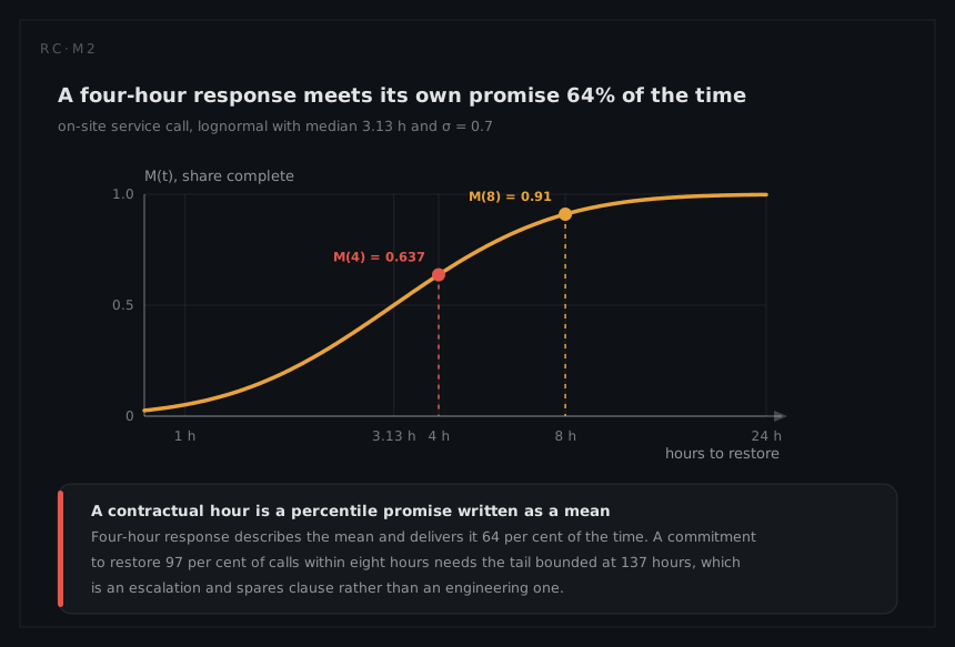
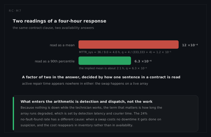
The 4 hours enters the availability model as a mean. Read as a contractual service level it is normally understood as a ceiling, and the gap between the two readings is a factor of two in the answer. Model dispatch as a lognormal with the canonical σ = 0.7 and work both.
If 4 hours is the mean, the median dispatch is 4 / e^0.245 = 3.13 hours and
M(4) = Φ(ln(4 / 3.13) / 0.7) = Φ(0.350) = 0.637
so barely 64% of calls are met inside four hours, and a customer reading that number as a commitment would consider the service broken. If 4 hours is the 90th percentile, then tmed = 4 / 2.452 = 1.63 hours and the mean is 2.08 hours. Single-controller unavailability follows from a mean life of 1 / (3.0 × 10⁻⁶) = 333,333 hours:
q = 4 / (333,333 + 4) = 1.2 × 10⁻⁵ against q = 2.08 / (333,333 + 2.08) = 6.3 × 10⁻⁶
The same three words produce two availability answers a factor of two apart, and the model quoted in this chapter silently took the weaker. Writing down which reading is intended, and buying the contract that matches it, is most of the maintainability work available on this system.
Detection has the same double edge. Telemetry and drive self-monitoring give 97% coverage, so 3% of failures reach the customer before the monitoring system. Rather than guess a latency, invert the question: for the effective restoration mean to double from 4 hours to 8, the undetected 3% would need to sit for
(8 − 0.97 × 4) / 0.03 = 4.12 / 0.03 = 137 h
which is under six days. On a system whose entire annual downtime budget is five minutes, a failure unnoticed for a working week is not an edge case in the tail; it is the mode that decides the year. The testability page works the coverage arithmetic that keeps the 3% small.
The arithmetic the repair time never enters
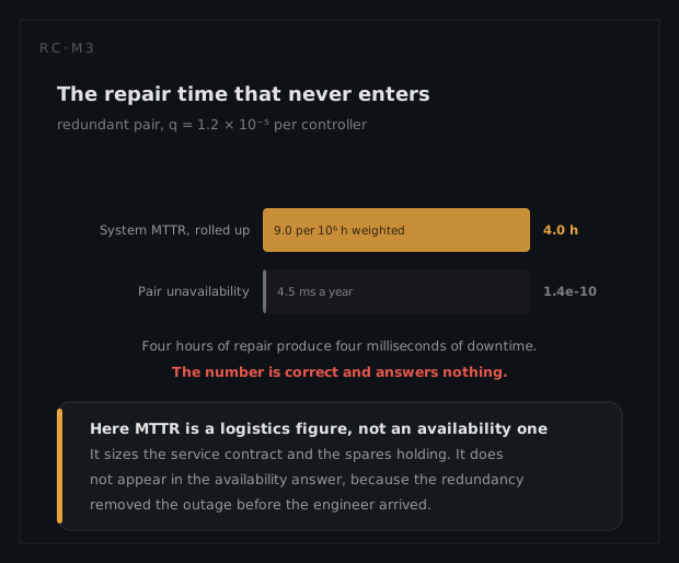
With independent repair the controller pair multiplies:
qpair = (1.2 × 10⁻⁵)² = 1.4 × 10⁻¹⁰
five orders of magnitude below the 10⁻⁵ unavailability budget the five-nines target allows, so the controller pair is not the constraint and no improvement to it is worth funding. The shared backplane and the shared firmware build are, because neither is duplicated and neither is covered by the multiplication.
The firmware point deserves the arithmetic. Five nines is 8,760 × 60 × 10⁻⁵ = 5.3 minutes of downtime a year, so a single disruptive update of 20 minutes spends 20 / 5.3 = 3.8 years of budget in one sitting. Four such updates a year is 80 minutes, giving 1 − 80 / 525,600 = 0.99985: between three and four nines, from planned maintenance alone, on an architecture whose unplanned unavailability is 1.4 × 10⁻¹⁰. Rolling, non-disruptive update is the single largest maintainability investment in the product, made in the architecture years before any array ships. The availability page prices it against the budget.
The bill arrives as parts
When a swap costs nothing in downtime it is performed on suspicion, and the cost reappears in inventory. No-fault-found on returned units runs at 24%, the highest of the eight rows, and it is structural rather than careless.
Controller-attributed failures arrive at 6.0 × 10⁻⁶ × 8,760 = 5.26 × 10⁻² per array-year, one every nineteen array-years. If those are the 76% of returns that are genuine, the return stream is 5.26 × 10⁻² / 0.76 = 6.92 × 10⁻² per array-year, so across a thousand installed arrays that is 69 controller returns a year, of which 17 are healthy. Each healthy return consumed a courier movement, a bench test, and a good board's residence on a shelf for weeks.
Set the chapter's three no-fault-found figures side by side (24% here, 21% on dealer brake ECUs, 17% on hospital infusion pumps) and the ordering follows the cheapness of the swap almost exactly. Cheap swaps are not free swaps; their price has moved from the downtime ledger to the warranty ledger, which is where this product's dominant service cost sits.
The lithium backup unit is the exception. Its thermal runaway mode makes removal a procedure with handling constraints, transport rules and a state-of-health check, so it is the one component nobody exchanges on suspicion. The item where safety writes the maintenance instruction is the item with no no-fault-found problem, and that is no coincidence: the procedure that makes the swap deliberate is the one that makes it correct. The safety page treats the hazard.
What the analysis tells the engineer to do
Buy the response contract on a percentile. A four-hour mean and a four-hour 90th percentile differ by a factor of two in q and by a large multiple in price; the availability model must state which it assumed.
Spend on detection latency, not repair speed. Coverage and alerting time are the only terms in the restoration model a design can move; the four hours belongs to a logistics network.
Treat planned maintenance as the availability risk it is. The largest single exposure is not a failure at all; it is a twenty-minute update.
What a different technique would have given
The conventional programme would run a demonstration in the MIL-STD-471 lineage: insert a representative sample of faults, have technicians of the specified skill level repair them under the specified conditions, and test the observed times against the requirement. Here it would produce hot-swap times measured in minutes, an MTTR inside any plausible requirement, and a clean pass.
It would also be measuring a quantity that is not in the availability equation. Every minute it recorded happens while the array is serving customers, so the demonstration would certify a property nobody experiences and produce no evidence about the terms that decide the outcome: detection coverage, alerting latency, dispatch percentile compliance and the disruptiveness of firmware updates. A demonstration that passes while the product misses its availability target has not been done badly; it has been aimed at the wrong term. The evidence this system needs is a coverage figure, a dispatch service-level report and an update strategy, none of which involves a stopwatch, and the maintainability prediction methods that would normally set the requirement have nothing to score.