

An electro-hydraulic brake actuator, two brake ECUs, four wheel-speed sensors, a backup hydraulic path and the regenerative torque interface, fitted to 200,000 vehicles driven 500 hours a year each. Repairs happen at dealers, are triggered by a diagnostic trouble code, and take an hour and a bit. None of that sounds like a maintainability problem worth a page.
It becomes one at scale. Two hundred thousand vehicles turn a modest repair time into a national capacity plan, and a capacity plan cannot be built on a mean. A service bay is booked in slots, and a slot is a commitment that a job will be finished by a stated time; whether it is depends entirely on the shape of the repair-time distribution and not at all on its average. This is the chapter's flagship page for fitting that shape, because it is the one system with enough work orders to fit it properly.
The technique, and why this one
A lognormal fitted by maximum likelihood to dealer work-order data, with the median, mean and percentile relations used to convert the fit into bay-scheduling decisions. Two features make the choice easy. The data exists: 41,000 corrective events a year, each with a labour-time record, which is more repair-time data than any other system in this chapter will see in its lifetime, and the FRACAS return stream is what delivers it. And the decisions being taken are percentile decisions, because nobody schedules a bay against a mean.
| Quantity | Model used | Value |
|---|---|---|
| Active repair time | lognormal fitted to work orders | mean 1.2 h, σ = 0.7, tmed = 0.94 h |
| Fault isolation outcome | two-branch mixture | 82% to a single replaceable unit |
| No-fault-found returns | binomial share of the return stream | 21% on brake ECUs |
| Parts logistics delay | deterministic delay | 21.6 h |
| Vehicle off road | additive downtime model | 33.6 h per incident |
| Event arrival rate | rate-and-exposure product | 41,000 events a year |
The σ = 0.7 is this chapter's canonical spread, and on this system it would not stay an assumption for long: with n = 41,000 records the standard error on a maximum-likelihood σ̂ is roughly σ / √(2n) = 0.7 / 286 = 0.002, so the shape parameter would be pinned to three decimal places while engineers were still arguing about the mean.
Fitting the repair time
The fit's natural parameter is the median, and the mean follows from it:
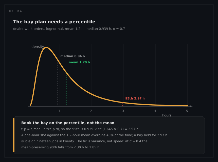
tmed = mean / e^(σ²/2) = 1.2 / e^0.245 = 1.2 / 1.2776 = 0.939 h = 56 min
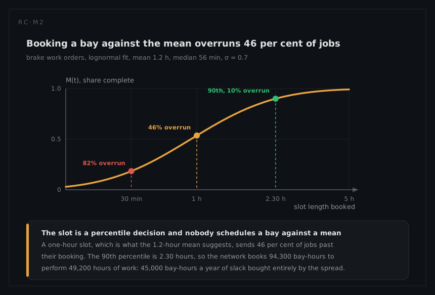
The typical brake job takes 56 minutes; the average takes 72. That 28% gap is not noise, it is the tail pulling the mean up, and it is the first thing a scheduler needs. The percentiles follow from tp = tmed × e^(zp·σ):
t₀.90 = 0.939 × e^(1.282 × 0.7) = 0.939 × 2.452 = 2.30 h
t₀.95 = 0.939 × e^(1.645 × 0.7) = 0.939 × 3.163 = 2.97 h
The maintainability function then answers what the booking system actually asks:
| Slot length | M(t) | Jobs that overrun |
|---|---|---|
| 30 min | Φ(ln(0.5 / 0.939) / 0.7) = Φ(−0.901) = 0.184 | 82% |
| 1 hour | Φ(ln(1.0 / 0.939) / 0.7) = Φ(0.090) = 0.536 | 46% |
| 2 hours | Φ(ln(2.0 / 0.939) / 0.7) = Φ(1.080) = 0.860 | 14% |
| 2.30 hours | 0.90 by construction | 10% |
A one-hour slot against a 1.2-hour mean fails 46% of the time, which every service manager knows empirically and no MTTR figure predicts. The honest specification is two numbers, MTTR = 1.2 h and Mmax(95%) = 2.97 h, and the second is what the network is built around.
What the schedule costs
The system runs at 410 per 10⁶ hours over 500 operating hours a year, giving 0.205 failures per vehicle-year and, across 200,000 vehicles, 41,000 corrective events a year. At 1.2 hours each the work content is 49,200 technician-hours. That count is deliberately larger than the 39,000 vehicle-off-road incidents the availability page works from: a dormant backup path found dead at the annual service occupies a bay and a technician exactly as a failure does, and only the customer's ledger gets to ignore it.
The work content is not what the network buys. Cut slots to the 90th percentile so nine jobs in ten finish inside their booking and the network books 41,000 × 2.30 = 94,300 bay-hours to perform 49,200 hours of work. Forty-five thousand bay-hours a year of scheduling slack, bought entirely by the σ = 0.7 spread, and no reduction in the mean recovers any of it. Cutting σ to 0.4 while leaving the mean alone moves the 90th percentile to (1.2 / e^0.08) × e^(1.282 × 0.4) = 1.108 × 1.671 = 1.85 hours and saves 41,000 × 0.45 = 18,500 bay-hours a year. Standardised procedures, better documentation and a consistently resolving diagnostic are variance interventions, and here variance is worth more than speed.
Where the customer's clock goes
Vehicle off road runs at 1.4 days, or 33.6 hours, of which 21.6 is parts logistics and 1.2 is the repair. The residual is
33.6 − 21.6 − 1.2 = 10.8 h
of booking, queueing, diagnosis handover and paperwork. The repair itself is 3.6% of the customer's lost time, the supply chain 64% and administration 32%. A programme aimed exclusively at the design competes for less than a twenty-fifth of the outcome. Both ledgers are real; they are owned by different departments, and the maintainability engineer's job is to say which is which rather than pretend one is the other. The availability page works the logistics side.
Ambiguity, and the parts it consumes
Fault isolation resolves to a single replaceable unit 82% of the time, so 18% of 41,000, or 7,380 events a year, begin with a group rather than an answer. In a two-unit group with equal priors the expected number of swaps is 1.5, drawing 3,690 additional parts a year for no fault at all.
The return stream shows the same effect from the other end. The two brake ECUs contribute 120 of the system's 410 per 10⁶ hours, so ECU-attributed events run at
41,000 × 120 / 410 = 12,000 events a year
If those are the 79% of returns that are genuine, the return stream is 12,000 / 0.79 = 15,190 units, of which 3,190 are no-fault-found. Each consumed 1.2 hours of bay time, for 3,830 technician-hours a year producing nothing, plus a part drawn from a 21.6-hour pipeline and a good unit sitting on a shelf until it is tested weeks later. The ambiguity estimate of 3,690 unnecessary parts and the warranty stream's 3,190 healthy returns are the same effect counted twice, and their agreement to within 15% is the best available evidence that the 82% isolation claim is roughly honest.
What the analysis tells the engineer to do
Fund diagnostic resolution ahead of wrench time. Resolution is the only input that improves elapsed time, parts consumption and warranty cost simultaneously: it shortens the isolation element, removes the 3,690 speculative swaps, and shrinks the tail that forces 2.30-hour slots. The testability analysis behind the 82% is a maintainability document in everything but name, and the testability page works the coverage arithmetic.
Specify the percentile, not the mean. A contract written on a 1.2-hour MTTR is met by a design whose 95th percentile is 2.97 hours and equally by one whose 95th is 1.6 hours, and the network pays a completely different price for the two.
Treat variance reduction as a design activity. Captive fasteners, keyed connectors, one-way fits and a procedure that cannot be performed in the wrong order all compress the tail rather than the median. They look like small changes on a 56-minute job and are worth tens of thousands of bay-hours across a fleet this size.
What a different technique would have given
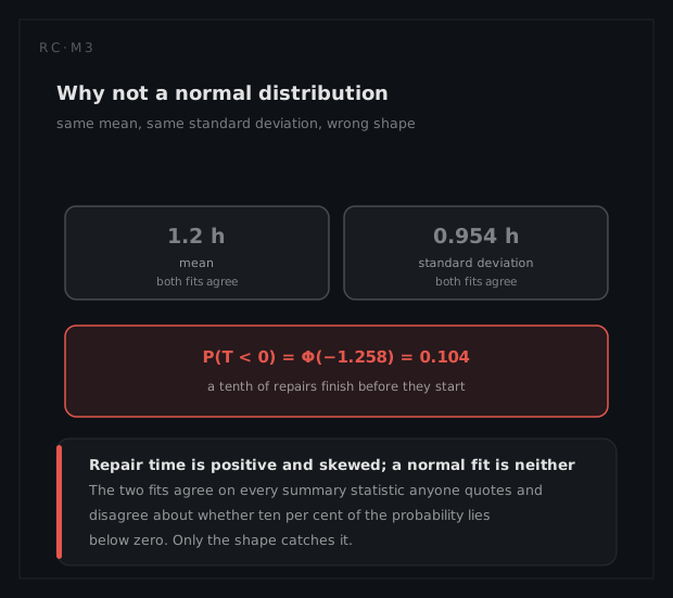
The obvious alternative is a normal distribution fitted to the same 41,000 records, which is effectively what any workshop system quoting a mean and a standard deviation produces. Matching the lognormal's first two moments gives
sd = mean × √(e^(σ²) − 1) = 1.2 × √0.632 = 1.2 × 0.795 = 0.954 h
and a normal with mean 1.2 and sd 0.954 fails immediately in a way that should end the discussion:
P(T < 0) = Φ((0 − 1.2) / 0.954) = Φ(−1.258) = 0.104
The model assigns 10.4% of its probability to repairs that finish before they start. It also mishandles the end that matters. Its 90th percentile is 1.2 + 1.282 × 0.954 = 2.42 hours, close enough to the lognormal's 2.30 to look acceptable; its 99th is 1.2 + 2.326 × 0.954 = 3.42 hours against the lognormal's 0.939 × 5.095 = 4.79. The normal truncates the long jobs, which are precisely the ones that overrun a bay, strand a customer overnight and generate the escalations a warranty budget is sized for. A symmetric distribution cannot describe an asymmetric process, and repair work is asymmetric because there is a floor on how fast a job can go and no ceiling on how slowly.
The exponential deserves a briefer note. With μ = 1 / 1.2 = 0.833 per hour it makes the availability algebra linear and is used for that alone. It is not fitted to this data and should not be quoted as a description of it, because readers downstream will not keep the distinction between a convenience model and a fitted one unless the report keeps it for them.