

One emergency diesel generator, its fuel oil system, starting air, the load sequencer and the output breaker, two trains per unit, standby duty, demanded only on loss of offsite power. Work is planned into the refuelling outage wherever it can be, and when it cannot, it happens under a clock written into the plant's technical specifications rather than into a maintenance contract.
That clock is why this machine ends the chapter. The allowed outage time for corrective work is 72 hours, and it is not a target and emphatically not a mean. It is a ceiling with a plant shutdown behind it, which makes the governing requirement a very high percentile of a distribution most programmes never characterise. A second constraint runs alongside with no clock at all: dose accumulated during the work is a first-class cost, ranked with elapsed time rather than beneath it.
The technique, and why this one
A lognormal repair-time model inverted against a regulatory percentile, so that the ceiling determines the permitted mean rather than the other way round, combined with a multi-attribute objective in which collective dose sits alongside duration. Every other page starts with a mean and asks what percentile follows; here the percentile is fixed by a licence condition and the question is what mean, and what spread, are compatible with it.
| Quantity | Model used | Value |
|---|---|---|
| Corrective repair time | lognormal, σ = 0.7 canonical, σ = 0.4 achievable | inverted from the ceiling |
| Allowed outage time | hard ceiling at a high percentile | 72 h |
| Support-system corrective demand | exponential, rates summed | 490 per 10⁶ h |
| Surveillance unavailability | deterministic, 12 outages a year | 2 h each |
| Latent exposure between tests | λT/2 | λDU = 45 per 10⁶ h, T = 730 h |
| Dose | task-analysis build-up, posture and position by element | no time equivalent |
Failure of the train itself is measured rather than predicted, at 3.0 × 10⁻³ per demand to start and 1.0 × 10⁻³ per hour to run, giving one train 2.67 × 10⁻² over a 24-hour mission and the pair 2.0 × 10⁻³ once common cause is admitted, as the reliability page works out. Those figures set how often the maintainability question is asked; they do not answer it.
The ceiling is a percentile, not a mean
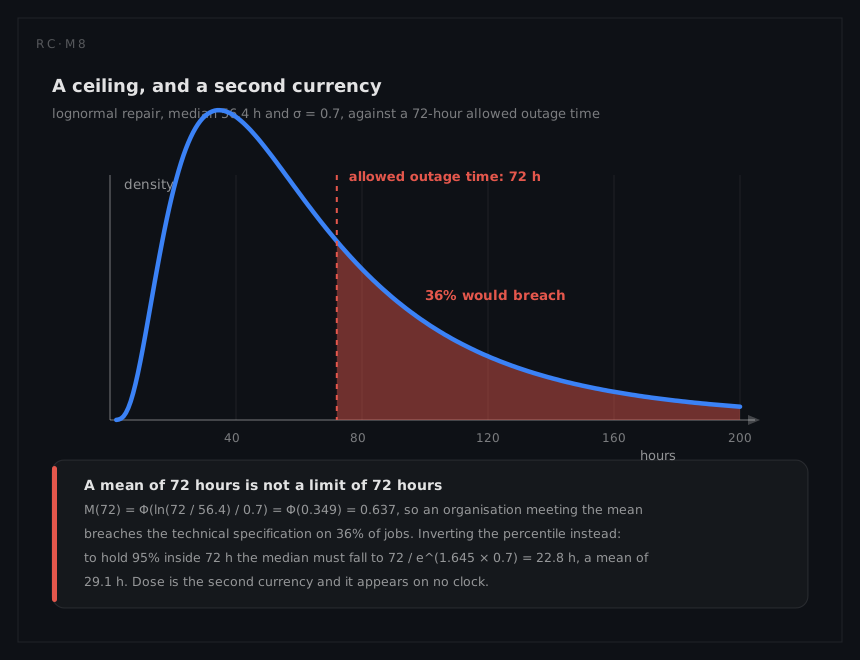
Suppose a programme takes the 72 hours at face value and plans to it as an MTTR. With a lognormal at σ = 0.7 the median is 72 / e^0.245 = 56.4 hours, so
M(72) = Φ(ln(72 / 56.4) / 0.7) = Φ(0.350) = 0.637
More than a third of corrective jobs would breach a technical specification limit. That is not a maintainability shortfall but a licence problem, arriving from an arithmetic mistake no review of the mean would surface.
Invert it properly. To meet the ceiling at the 95th percentile,
tmed = 72 / e^(1.645 × 0.7) = 72 / 3.163 = 22.8 h and mean = 22.8 × e^0.245 = 29.1 h
To meet it at the 99th percentile, as the consequence arguably deserves,
tmed = 72 / e^(2.326 × 0.7) = 72 / 5.095 = 14.1 h and mean = 14.1 × e^0.245 = 18.1 h
The same limit therefore implies a planning mean of 72, 29 or 18 hours depending entirely on a confidence the specification does not state and the maintenance organisation must choose. A factor of four in the design target hides inside an unstated percentile. Planning against 18 hours looks nothing like planning against 72: parts are pre-staged, the sequence is rehearsed, contingency branches are agreed at the outset, and a job whose credible worst case might exceed the ceiling is not started until an outage window can cover it. This is the mean-versus-percentile trap with a regulator attached.
Variance is cheaper than speed
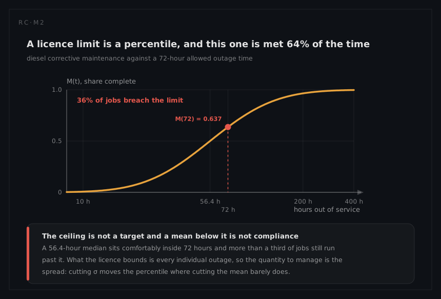
The other lever is spread, and here it is the cheaper one. Hold the 95th percentile at 72 hours and cut σ from 0.7 to 0.4:
tmed = 72 / e^(1.645 × 0.4) = 72 / 1.931 = 37.3 h and mean = 37.3 × e^(0.4²/2) = 37.3 × 1.083 = 40.4 h
The permitted mean rises from 29.1 hours to 40.4, so a crew that has made its work predictable may be eleven hours slower on average and still meet the same limit at the same confidence. Nothing in that trade requires a faster tool or a better access route. It requires pre-staged parts, a rehearsed sequence, a written contingency for each credible complication and a supervisor empowered to stop rather than improvise. Rehearsal buys percentile margin without touching the mean, and where the requirement is a percentile that is the higher-yield investment.
Three unavailability terms, and which one maintainability owns
The train is unavailable for three reasons, and their ranking is not the expected one.
| Contribution | Arithmetic | Value |
|---|---|---|
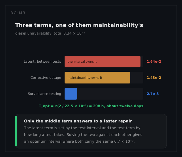
| Latent failures between tests | 45 × 10⁻⁶ × 730 / 2 | 1.64 × 10⁻² |
| Corrective work under the AOT clock | 4.29 events/y × 29.1 h / 8,760 | 1.43 × 10⁻² |
| Surveillance starts | 12 × 2 h / 8,760 | 2.74 × 10⁻³ |
| Total | 3.34 × 10⁻² |
The corrective term is derived rather than quoted. The support systems (fuel oil at 250, starting air at 180 and the load sequencer at 60 per 10⁶ hours) sum to 490 per 10⁶ hours, so the train generates 490 × 10⁻⁶ × 8,760 = 4.29 corrective demands a year, and at the 29.1-hour planning mean that is 125 hours of unavailability a year.
Two things follow. Corrective maintainability is the second-largest unavailability term here, within 15% of the latent term and five times the surveillance term, which is not where a casual reading of a standby system would put it. And the percentile discipline pays twice: the 99th-percentile target with its 18.1-hour mean drops the corrective term to 4.29 × 18.1 / 8,760 = 8.85 × 10⁻³, cutting total unavailability by 16% as a side effect of a compliance decision.
The latent term is the largest and belongs to another chapter, but the trade is settled with maintenance numbers. Halving the test interval to 365 hours takes it to 8.2 × 10⁻³ while doubling the surveillance term to 5.5 × 10⁻³, a net gain. The sum of the two is minimised where
d/dT [ 22.5 × 10⁻⁶ · T + 2 / T ] = 0 → T = √(2 / 22.5 × 10⁻⁶) = 298 h
which is fortnightly, and delivers 1.34 × 10⁻² against the monthly regime's 1.92 × 10⁻²: a 30% improvement. Practice does not chase it, because each start wears the machine and costs the crew dose. The testability page works the detection side in full.
The constraint with no clock
Dose reorders everything above. The objective is not minimum duration but minimum collective dose subject to completing inside the ceiling at the required confidence. A layout change that saves twenty minutes at the price of an awkward posture in a higher-dose area is a good trade in seven of these eight rows and a bad one here.
That is why the task analysis, rather than the repair-time prediction, becomes the governing document. A prediction produces a duration; a task analysis produces a sequence of elements each with a location, a posture, a duration and a headcount, which is what a dose estimate consumes, and it is the only maintainability artefact that can be optimised against two currencies at once.
What the analysis tells the engineer to do
State the percentile in the maintenance basis. The 72 hours is given; the confidence at which it must be met is worth a factor of four in the planning target, and leaving it unstated means it gets chosen implicitly by whoever writes the job card.
Invest in variance, not velocity. Pre-staging, rehearsal and pre-agreed contingencies are worth eleven hours of permitted mean at the same compliance level, and cost less than any hardware change.
Count the corrective term. At 1.43 × 10⁻² it rivals the latent exposure that gets all the analytical attention, and it is the only one of the three a maintenance organisation can move without a licence amendment.
Optimise dose and time together. Ranking the levers by elapsed time alone recommends changes that increase collective dose, and no exchange rate in the specification will catch the error.
What a different technique would have given
The conventional approach is an MTTR requirement backed by an exponential repair model, and it fails here in two independent ways.
Specifying the mean is the larger error. A 72-hour MTTR is met by an organisation whose jobs breach the technical specification 36% of the time, and the requirement reports itself as satisfied throughout. There is no version of that outcome in which the specification did its job.
The exponential model is the smaller error and points the other way. With mean m it gives M(72) = 1 − e^(−72/m), so achieving 95% compliance would demand m = 72 / ln 20 = 24.0 hours against the lognormal's 29.1: a target 17% tighter than necessary and correspondingly more expensive in pre-staging and standby crew. Read at 29.1 hours it predicts an 8.4% breach rate where the fitted shape predicts 5%. Neither error is enormous alone, and the reason to care is that they compound in opposite directions with the mean-specification error, so a programme making both cannot tell which way it is wrong. Where a limit is a licence condition, the distribution is not a modelling refinement; it is the difference between compliance and a finding.