

An emergency diesel generator, its fuel oil system, starting air, a load sequencer and an output breaker, two trains per unit, demanded only when offsite power is lost. Every other system in this chapter has some continuous signal a monitor can watch. This one spends its entire life switched off, and no instrument yet devised will tell you whether a diesel that has not run for a month will start when it is asked.
There is exactly one test that answers the question, and it is to start the machine. That single fact makes the surveillance programme the whole of the testability provision, converts an entirely latent population into a periodically revealed one, and moves the design question from "can we detect it" to "how often can we afford to look". The test is not free, and its two prices move in opposite directions.
The technique, and why this one
Periodic demand testing analysed as an interval optimisation: the latent exposure λT/2 that falls with a shorter interval, set against the test-induced unavailability ttest/T that rises with it, minimised at T = √(2·ttest/λ). The technique follows from the machine. A dormant item has no coverage between tests, so the only lever is the interval; and unlike a shutdown valve, this item's test takes it out of service while it runs, so shortening the interval buys latent exposure back at a price. Where both effects exist, the answer is an optimum rather than a direction.
| Quantity | Value | Model used | Test means |
|---|---|---|---|
| Failure to start | 3.0 × 10⁻³ per demand | binomial, per demand, estimated from 18 failures in 6,000 surveillance demands | the surveillance start, and nothing else |
| Failure to run | 1.0 × 10⁻³ per hour | exponential over the 24-hour mission | the surveillance run |
| Fuel oil system | 250 per 10⁶ h | constant λ | day tank level, pressure, water-in-fuel alarms |
| Starting air | 180 per 10⁶ h | constant λ | receiver pressure, compressor run status |
| Load sequencer | 60 per 10⁶ h | constant λ, dormant logic | limited self-test only |
| Dangerous undetected between tests | 45 per 10⁶ h | roll-up of what monitoring cannot reach | surveillance start at T = 730 h |
The split between a per-demand probability and a per-hour rate is the shape of the machine, not a refinement: a start failure is binomial and does not grow with mission length, while a run failure is a rate and does. Over a 24-hour mission,
Frun = 1 − e^(−1.0 × 10⁻³ × 24) = 1 − e^(−0.024) = 2.37 × 10⁻²
Ftrain = 3.0 × 10⁻³ + 2.37 × 10⁻² = 2.67 × 10⁻²
and the reliability page carries that through to the pair, where a common-cause fraction of 0.05 gives 2.0 × 10⁻³ and the common-cause term dominates.
What continuous monitoring can and cannot reach
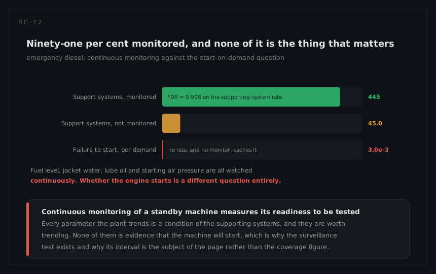
The standby state is not entirely unwatched. Fuel level, air receiver pressure, jacket water temperature, battery charge and lube oil level are all instrumented, and they cover a large share of the supporting systems:
| Item | λ per 10⁶ h | Detected continuously | Undetected λ |
|---|---|---|---|
| Fuel oil system | 250 | 92.0% | 20.0 |
| Starting air | 180 | 90.0% | 18.0 |
| Load sequencer | 60 | 88.3% | 7.0 |
| Total | 490 | 45.0 |
FDR = (490 − 45.0) / 490 = 445 / 490 = 0.908
Ninety-one per cent of the supporting-system rate is watched, and it buys almost nothing on its own, because the 3.0 × 10⁻³ per demand that dominates the risk model is not in this table at all. Nothing instrumented tells you that the governor will pick up, that the fuel rack will move, that the air start motor will engage or that the sequencer will load the buses in order. The dominant failure mode of a standby machine is the transition itself, and a transition can only be tested by making it happen. The 45 per 10⁶ hours above is therefore the residual the surveillance start reveals, not the whole of what it reveals.
The interval, with costs on both sides
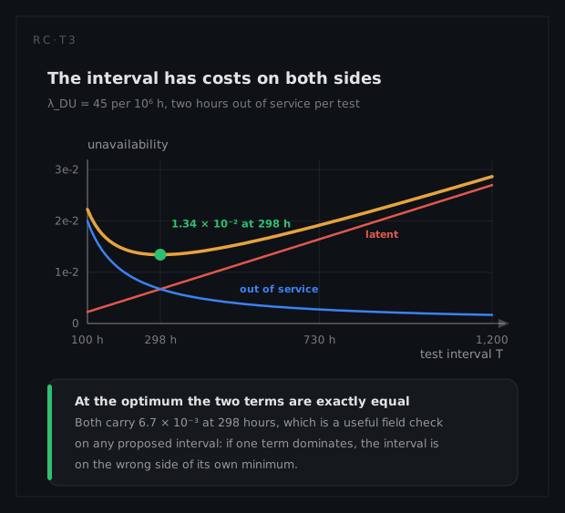
Between tests the residual accumulates, and the average latent unavailability is
Ulatent = λDU × T / 2 = 45 × 10⁻⁶ × 730 / 2 = 1.6 × 10⁻²
Each surveillance start also takes the train out of service for two hours while it runs, which is an unavailability of
Utest = ttest / T = 2 / 730 = 2.7 × 10⁻³
and the total at the monthly interval is
U(730) = 1.6 × 10⁻² + 2.7 × 10⁻³ = 1.9 × 10⁻²
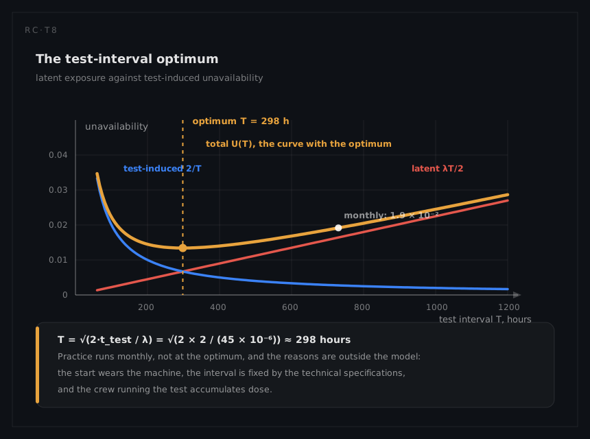
One term falls with T and the other rises as 1/T, so the sum has a minimum. Differentiating
U(T) = λT/2 + ttest/T
dU/dT = λ/2 − ttest/T² = 0
gives the classic result
Topt = √(2·ttest / λ) = √(2 × 2 / (45 × 10⁻⁶)) = √88,889 = 298 h
about twelve days. At that interval each term is 6.7 × 10⁻³ and the total is 1.34 × 10⁻², a 30% improvement on the monthly figure. Note the general property the algebra delivers: at the optimum the latent term and the test-induced term are exactly equal, which is a useful field check on any proposed interval without recomputing anything.
Practice does not chase the optimum, and the reasons are the honest limits of a purely mathematical treatment. The interval is fixed by the technical specifications. A surveillance start wears the machine, so the assumption that testing costs only its two hours is false at ten-day intervals. And the crew accumulates dose, which the maintainability page treats as a first-class constraint alongside time. The value of the calculation is the shape it reveals rather than the number: anyone arguing for a longer interval trades against a term that grows linearly, and anyone arguing for a shorter one against a term that grows without limit as T falls.
The test is also the measuring instrument
There is an asymmetry here that no other row in this chapter has. The surveillance programme is not only the mitigation, it is the evidence. The 3.0 × 10⁻³ the whole risk model rests on comes from counting the outcomes of surveillance starts:
p̂ = 18 / 6,000 = 3.0 × 10⁻³
At twelve demands per train-year, six thousand demands represents 500 train-years of accumulated surveillance, and the estimate still carries a bound worth quoting:
pupper = χ²(0.95; 2r + 2) / (2n) = 53.4 / 12,000 = 4.4 × 10⁻³
so the honest statement is 3.0 × 10⁻³ with a 95% upper bound of 4.4 × 10⁻³, and a probabilistic risk assessment should be run at both. The test therefore does three jobs at once: it reduces the latent exposure, it reveals the individual faults, and it produces the population statistic that says how much risk remains. Lengthen the interval and all three degrade together, which is a coupling that a purely availability-based interval argument misses entirely.
One further pressure deserves naming rather than pretending away. The technical specifications allow 72 hours for corrective work, and that clock begins when the fault is found, not when it occurred. Discovering a problem therefore starts a countdown a plant under commercial pressure would rather not start. Every testing programme carries some version of that bias, and good practice answers it by writing the acceptance criteria before the test and keeping the person who judges the result separate from the person who owns the outage.
What the analysis tells you to do
Instrument what can be instrumented, and be clear that it is worth 45 per 10⁶ hours rather than the risk model. Fuel water content, air receiver leak-down rate and battery impedance are cheap monitors that shrink the residual the interval has to work on, and shrinking λDU pushes Topt outward: at 30 per 10⁶ hours the optimum moves to √(2 × 2 / 30 × 10⁻⁶) = 365 hours, so better monitoring buys a longer permissible interval rather than merely a lower number.
Make the surveillance start earn its full diagnostic value while it is running. A start that only proves the machine started throws away the run: exhaust temperature spread, cylinder pressures, governor response time and load acceptance are all measurable in the two hours already being paid for, and trending them converts a pass/fail demand test into a condition-monitoring stream. Finally, treat the two hours as a design parameter and not a constant. Halving the test outage moves the optimum to √(2 × 1 / 45 × 10⁻⁶) = 211 hours and lowers the achievable minimum, so a procedure change that lets the train be recovered to standby faster is worth as much as an instrument.
What a different technique would have given
The alternative that engineers reach for is appealing and wrong here: instrument the machine thoroughly enough that periodic starting becomes unnecessary. Jacket water temperature, prelube pressure, fuel quality, air pressure, battery state and governor position, all continuously monitored, with an alarm on any deviation.
Work out what it delivers. It attacks the 490 per 10⁶ hours of supporting-system rate, where coverage is already 90.8%, so the best case is that the residual 45 falls towards zero. It does nothing about the start transition, because nothing in that list demonstrates that the machine turns, fires, comes up to speed and takes load in sequence. The 3.0 × 10⁻³ per demand would remain unmeasured, and the risk assessment would lose its only empirical input and revert to a handbook figure with no confidence bound. Meanwhile, with the interval stretched to a year on the strength of the monitoring, the residual that monitoring cannot reach would carry
Ulatent = 45 × 10⁻⁶ × 8,760 / 2 = 2.0 × 10⁻¹
more than a factor of twelve worse than the monthly figure. Continuous monitoring and demand testing are not substitutes; they address disjoint populations, and on a standby machine the population that monitoring cannot address is the one the safety case is about.