

An emergency diesel generator, its fuel oil system, starting air, a load sequencer and an output breaker, two trains per unit, sitting idle until offsite power is lost. The hazard is station blackout, and this machine is one layer of defence among several that stand between the plant and it. That last clause changes what the analysis is for. Nobody claims the diesel train makes the plant safe. The claim is that it is a layer, that the layers together hold, and that its unavailability is a quantity another model consumes.
It is the only system in this chapter whose safety target does not belong to the system being analysed. The number produced below goes into a probabilistic risk assessment as a direct contributor to core damage frequency, alongside layers with nothing to do with electrical power, and it is judged there rather than here. That discipline is useful: improving the diesel is worth precisely what it moves the plant figure, and no more.
The technique, and why this one
A fault tree over the pair, with each train quantified as a per-demand probability plus a per-hour rate, a beta-factor common-cause basic event coupling the two, and a latent term from the surveillance interval. Two features of the machine force it. First, it fails in two physically distinct ways that no single measure captures: it can fail to start when asked, and it can fail while running. Second, the trains are nominally independent and are not, so the tree needs a basic event that lives in both branches, which is something only a fault tree with common cause can express.
| Quantity | Model | Value | Basis |
|---|---|---|---|
| Failure to start | per-demand binomial | 3.0 × 10⁻³ | 18 failures in 6,000 surveillance demands |
| 95% upper bound on the above | chi-square | 4.4 × 10⁻³ | χ²(0.95; 38)/12,000 |
| Failure to run | exponential, 24-hour mission | 1.0 × 10⁻³ per hour | |
| Fuel oil system | exponential | 250 per 10⁶ h | supporting system |
| Starting air | exponential | 180 per 10⁶ h | supporting system |
| Load sequencer | exponential | 60 per 10⁶ h | supporting system |
| Common cause between trains | beta factor | β = 0.05 | design, crew, fuel, procedures, environment |
| Undetected dangerous rate between tests | λT/2 | 45 per 10⁶ h, T = 730 h | monthly surveillance |
| Test-induced unavailability | outage fraction | 2 h per 730 h | the surveillance start itself |
| Allowed outage time for corrective work | technical specifications | 72 h | this sector's limit |
One train, two clocks
The start failure is a probability per demand and does not grow with mission length. The run failure is a rate per hour and does. Over the 24-hour mission:
Frun = 1 − e^(−1.0 × 10⁻³ × 24) = 1 − e^(−0.024) = 2.37 × 10⁻²
qtrain = 3.0 × 10⁻³ + 2.37 × 10⁻² = 2.67 × 10⁻²
Keeping the two separate is not fastidiousness. A six-hour blackout is dominated by the start term and a week-long one by the run term, and a model that collapsed them into a single mean time between failures would get the mission-length sensitivity wrong in both directions. The supporting systems, fuel oil at 250, starting air at 180 and the sequencer at 60 per 10⁶ hours, sit underneath both terms and are what most of the 2.67 × 10⁻² is actually made of.
The order-one cut set the architecture was built to avoid
Two trains treated as independent multiply:
qpair (independent) = (2.67 × 10⁻²)² = 7.1 × 10⁻⁴
They are not independent. Both trains share a design, a maintenance organisation, a fuel supply, a set of procedures, a building and an ambient environment. The beta factor splits each train's probability into an independent part (1 − β)q and a part βq attributed to causes that fail both:
independent part = ((1 − 0.05) × 2.67 × 10⁻²)² = (2.537 × 10⁻²)² = 6.4 × 10⁻⁴
common-cause part = 0.05 × 2.67 × 10⁻² = 1.3 × 10⁻³
qpair = 6.4 × 10⁻⁴ + 1.3 × 10⁻³ = 2.0 × 10⁻³
Read that as cut sets rather than as a sum and the finding is sharper. The independent part is the order-two cut set {train A, train B}. The common-cause part is a single basic event that fails both, which is an order-one cut set, and it is twice the size of the order-two one. The aircraft elsewhere in this chapter is forbidden an order-one cut set by rule. Here one exists, it is admitted by name, and it dominates. The honest pair value is 2.8 times worse than multiplication promised.
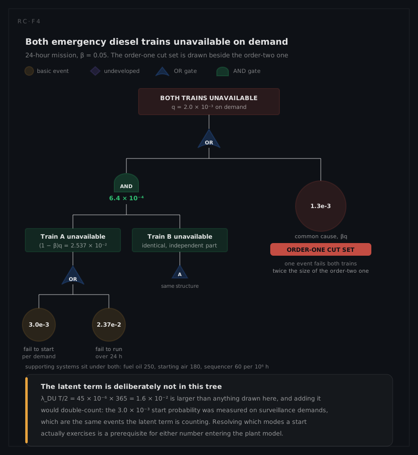
Drawn out, the asymmetry is impossible to miss and that is the point of drawing it. A basic event connected directly to the top OR gate is, by definition, an order-one cut set: nothing else has to happen. The two trains are three levels down and need each other. In a fault tree the depth of an event is a statement about how much has to go wrong to reach the top, and here the largest contributor is also the shallowest.
Each train expands to an OR of its two failure modes, with the supporting systems underneath both: fuel oil at 250, starting air at 180 and the load sequencer at 60 per 10⁶ hours. Train B carries a transfer triangle rather than a second copy, which is honest here in a way it would not be on the aircraft: the two diesel trains really are structurally identical, and saying so is exactly the assumption the β on the right is charging for.
One term is deliberately absent. The latent contribution λDU T / 2 = 45 × 10⁻⁶ × 365 = 1.6 × 10⁻² is larger than everything in the tree combined, and putting it in would double-count, because the 3.0 × 10⁻³ failure-to-start probability was measured on surveillance demands and those are the same events the latent term counts. An analyst who adds every available number gets a worse answer than one who works out which numbers are estimates of the same thing. The surveillance section below returns to it.
What a third diesel is worth, and what it is not
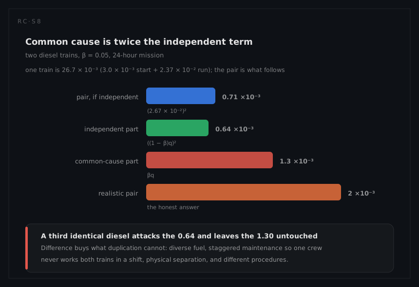
The beta-factor model answers the capital question directly. Add a third identical train and the independent part cubes while the common-cause part does not move:
independent part = (2.537 × 10⁻²)³ = 1.63 × 10⁻⁵
qtriple = 1.3 × 10⁻³ + 1.63 × 10⁻⁵ = 1.32 × 10⁻³
a factor of 1.5 on the pair, for a nine-figure item. And the limit is worse than that comparison suggests: as identical trains are added the independent part vanishes and the total tends to βq = 1.3 × 10⁻³ exactly. No quantity of identical hardware can get below 1.3 × 10⁻³, because the term that survives is the one that does not care how many there are.
Attack β instead. At β = 0.01 the same two trains give
independent part = ((0.99) × 2.67 × 10⁻²)² = (2.643 × 10⁻²)² = 7.0 × 10⁻⁴
common-cause part = 0.01 × 2.67 × 10⁻² = 2.67 × 10⁻⁴
qpair = 9.7 × 10⁻⁴
a factor of 2.1 on the pair from two trains, better than the third diesel bought, with an asymptote of 2.67 × 10⁻⁴ rather than 1.3 × 10⁻³. Diverse fuel supplies, staggered maintenance so one crew never works both trains in the same shift, physical and fire separation, different procedures and dissimilar starting arrangements all attack β itself. Difference buys more than duplication, and once a shared cause is admitted the arithmetic says so unambiguously. The independence assumptions that make a low β credible are the subject of the systems chapter.
Where the uncertainty actually is
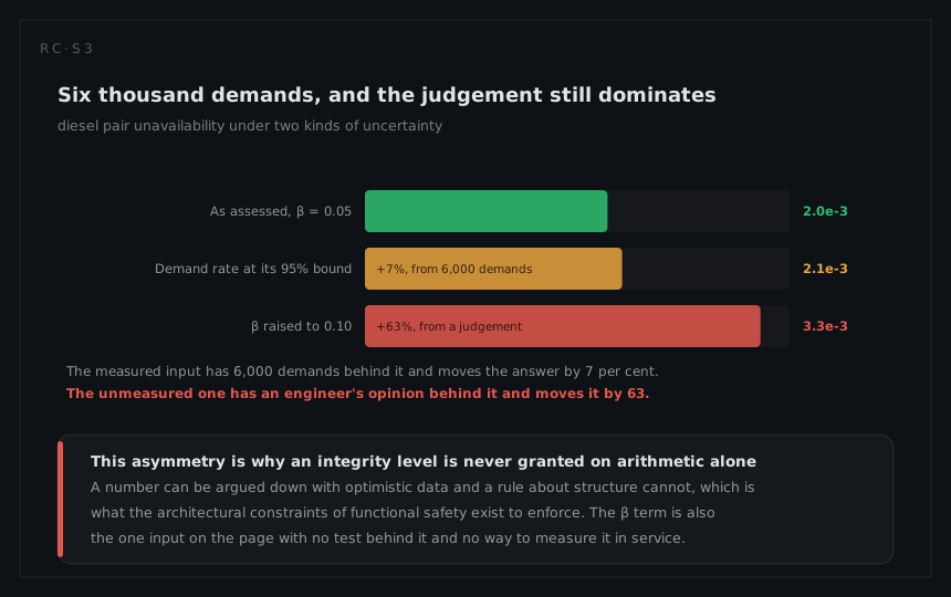
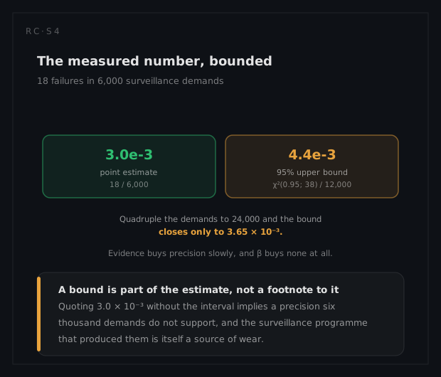
With 18 failures in 6,000 demands the start probability is measured rather than predicted, and the estimate carries a bound:
pupper = χ²(0.95; 2r + 2)/(2n) = χ²(0.95; 38)/12,000 = 53.4/12,000 = 4.4 × 10⁻³
Run the pair at the bound. The single train becomes 4.4 × 10⁻³ + 2.37 × 10⁻² = 2.81 × 10⁻², the independent part ((0.95)(2.81 × 10⁻²))² = 7.1 × 10⁻⁴, the common-cause part 0.05 × 2.81 × 10⁻² = 1.41 × 10⁻³, and the pair 2.1 × 10⁻³: a seven per cent increase on 2.0 × 10⁻³.
Now perturb β by the same kind of margin. At β = 0.10 the common-cause part is 2.67 × 10⁻³, the independent part ((0.90)(2.67 × 10⁻²))² = 5.8 × 10⁻⁴, and the pair 3.25 × 10⁻³, a 63 per cent increase. Seven per cent against sixty-three. The uncertainty that matters is β, not p, and β is the parameter with no 6,000 demands behind it. Effort spent accumulating more surveillance data refines the term the answer is least sensitive to, and the same chi-square machinery seen on the reliability page is worth running for exactly this reason: to find out which uncertainty is worth reducing.
The surveillance paradox, with an optimum
Between tests the train accumulates dangerous undetected failures at 45 per 10⁶ hours, and on a monthly interval the average latent unavailability is
λDU × T / 2 = 45 × 10⁻⁶ × 730 / 2 = 45 × 10⁻⁶ × 365 = 1.6 × 10⁻²
which is the largest single term on this page, sixty per cent of the whole single-train figure. Before it is used, note a trap the two estimates set for each other. The measured failure-to-start probability of 3.0 × 10⁻³ came from surveillance demands, and a surveillance demand reveals precisely the failures the latent term is counting. The two are, at least partly, estimates of the same thing, and adding them double-counts. They differ by a factor of 5.3, and resolving which modes the start exercises and which it does not is a prerequisite for either number entering the plant model.
The test itself is not free. Each surveillance start takes the train out of service for two hours, giving 2/730 = 2.7 × 10⁻³ of unavailability in its own right. Total unavailability as a function of interval is therefore λDU·T/2 + τ/T with τ = 2 h, and it has a minimum:
Topt = √(2τ / λDU) = √(4 / 45 × 10⁻⁶) = √88,889 = 298 h
about a fortnight. At that interval the latent term is 45 × 10⁻⁶ × 149 = 6.7 × 10⁻³ and the test-induced term is 2/298 = 6.7 × 10⁻³, equal as the optimum requires, for a total of 1.34 × 10⁻² against the monthly total of 1.6 × 10⁻² + 2.7 × 10⁻³ = 1.87 × 10⁻², a 28 per cent improvement. Practice does not go there, and the reasons are real and absent from the formula: every start wears the machine, and the crew running the test accumulates dose. The testability column works the trade from the detection side.
The 72-hour allowed outage time falls out of the same arithmetic. With one train out the pair's unavailability is the single train's 2.67 × 10⁻² rather than 2.0 × 10⁻³, a factor of 13. One full 72-hour outage a year raises the annual average from 2.0 × 10⁻³ to
(72/8,760) × 2.67 × 10⁻² + (1 − 72/8,760) × 2.0 × 10⁻³ = 2.2 × 10⁻⁴ + 1.98 × 10⁻³ = 2.2 × 10⁻³
a ten per cent increase. A limit on corrective work is a risk-informed number, not an arbitrary one, and it exists because a layer removed for maintenance is a layer that is not there.
What a different technique would have given
Model the pair with a reliability block diagram and the two trains sit in parallel, multiply, and report 7.1 × 10⁻⁴: 2.8 times better than the truth, and better for a structural reason. A block diagram has no notation for an event that belongs to two blocks simultaneously, so the order-one cut set that dominates this system simply cannot be drawn. It has a second problem too: a block carries a rate, and this machine's most likely failure is a per-demand probability, so the 3.0 × 10⁻³ would either be lost or smeared into an hourly figure that misrepresents every mission length except the one it was tuned to.
A Markov model is the more sophisticated alternative and is a genuine improvement in one respect: it handles the repair coupling, the 72-hour outage window and the surveillance interval as transitions rather than as bolt-on corrections, and it would produce the availability arithmetic above more elegantly. It does not touch the problem that matters, because β is a modelling assumption about shared causes, not a state in a state space. Every technique on this page is downstream of one judgement about how alike two machines are, and no amount of analytical machinery substitutes for making that judgement well.