

A standby diesel generator, its fuel oil system, starting air, a load sequencer and an output breaker, two trains per unit, demanded only when offsite power is lost. Every other page in this chapter has predicted or fitted a rate from a design or a return stream. This machine is tested so relentlessly that its reliability can simply be measured, and the page is about what changes when it can.
The technique, and why this one
A per-demand binomial estimate and a per-hour exponential estimate, both taken from surveillance records, combined in a fault tree with a beta-factor common cause, and quoted with a confidence bound. Two features of this machine force the approach. First, it can fail in two physically distinct ways that no single measure captures: it can fail to start when asked, and it can fail while running. Second, monthly surveillance starts across a fleet of similar machines over decades produce enough demands to estimate the start probability directly, rather than predicting it.
| Measure | Value | Basis |
|---|---|---|
| Failure to start, per demand | 3.0 × 10⁻³ | 18 failures in 6,000 surveillance demands |
| Failure to run, per hour | 1.0 × 10⁻³ | exponential over the 24-hour mission |
| Fuel oil system | 250 per 10⁶ h | supporting system, exponential |
| Starting air | 180 per 10⁶ h | supporting system, exponential |
| Load sequencer | 60 per 10⁶ h | supporting system, exponential |
Two clocks in one machine
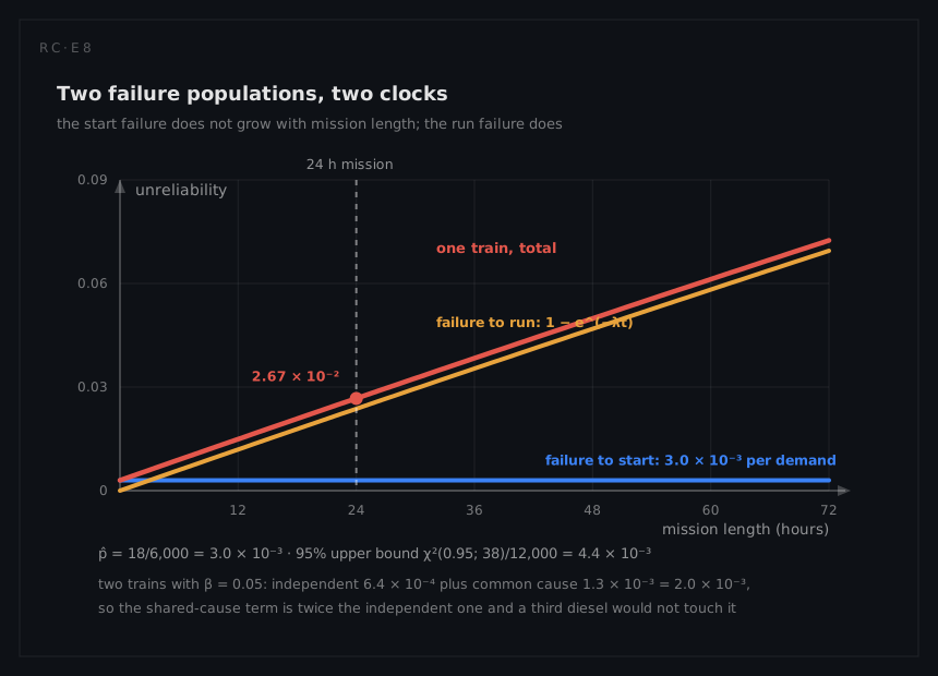
The start failure is a probability per demand: the machine is asked to start, and it either does or it does not. That is a binomial quantity and it does not depend on how long the mission is. The run failure is a rate per hour, and over a 24-hour mission it contributes
Frun = 1 − e^(−1.0 × 10⁻³ × 24) = 1 − e^(−0.024) = 2.37 × 10⁻²
so one train's unreliability over the mission is
Ftrain = 3.0 × 10⁻³ + 2.37 × 10⁻² = 2.67 × 10⁻²
That sum approximates the product 0.997 × e^(−0.024) = 0.97336, overstating the exact 2.664 × 10⁻² by the cross-term 7.1 × 10⁻⁵, which errs the safe way.
Collapsing these into a single MTBF, as an unwary analyst might, destroys the distinction. It would also get the mission-length sensitivity wrong in both directions: a one-hour mission is dominated by the start term, a week-long station blackout is dominated by the run term, and only a model that keeps them separate answers both.
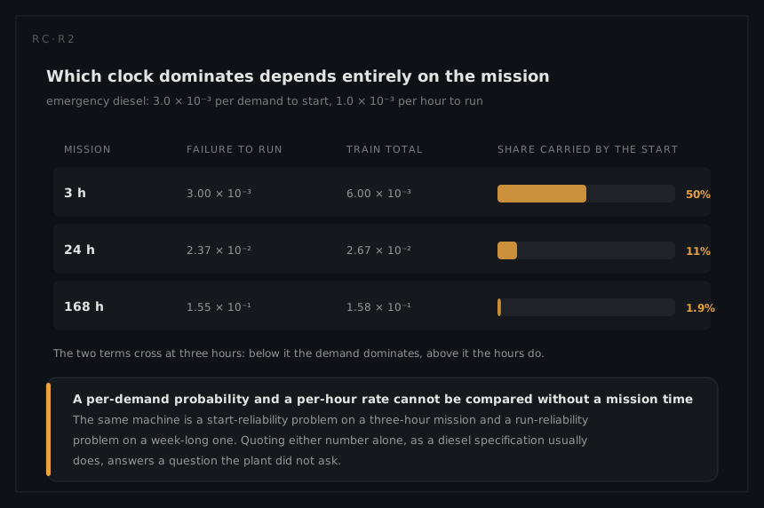
The two are equal where 1 − e^(−1.0 × 10⁻³ t) = 3.0 × 10⁻³:
tcross = −ln(0.997) / 1.0 × 10⁻³ = 3.0 h
| Mission | Frun | Ftrain | Start share |
|---|---|---|---|
| 3 h | 3.00 × 10⁻³ | 6.00 × 10⁻³ | 50% |
| 24 h | 2.37 × 10⁻² | 2.67 × 10⁻² | 11% |
| 168 h | 1.55 × 10⁻¹ | 1.58 × 10⁻¹ | 1.9% |
The start term carries half the answer at three hours and a fiftieth of it over a week.
What the run rate is made of
The 1.0 × 10⁻³ per hour is not one item. Three supporting systems sit underneath it, and a series chain multiplies survivals:
| Contributor | λ per 10⁶ h | R over 24 h |
|---|---|---|
| Fuel oil system | 250 | e^(−0.00600) = 0.99402 |
| Starting air | 180 | e^(−0.00432) = 0.99569 |
| Load sequencer | 60 | e^(−0.00144) = 0.99856 |
| In series | 490 | 0.98831 |
Fsupport = 1 − 0.98831 = 1.17 × 10⁻² and MTBFsupport = 10⁶ / 490 = 2,041 h
Just under half the run term is fuel, air and sequencer rather than the diesel, leaving 510 per 10⁶ hours for engine, alternator and breaker. Two other columns consume the same 490, read there as a standby calendar-hour rate rather than a running-hour one: it becomes 4.29 corrective demands a year (490 × 10⁻⁶ × 8,760) on the maintainability page and splits into 445 that instruments reach and 45 that only a start reveals on the testability page.
An engine that never accumulates hours
A diesel is exactly the sort of machine that gets a Weibull elsewhere in this chapter. The compressor train fits its turbine hot section at β = 3.1 and η = 52,000 hours, and is right to: it runs 8,760 hours a year and reaches η in 52,000 / 8,760 = 5.9 years, so its hazard genuinely climbs. This machine runs twelve times a year for two hours, 24 hours a year and 960 over a forty-year life, against a mean run life of 1,000 hours and a tenth percentile of
t10 = −ln(0.9) / 1.0 × 10⁻³ = 105 h
Reaching the turbine's 52,000 hours would take 52,000 / 24 = 2,167 years. The exponential is right here not because a diesel does not wear, but because it is never given the hours in which to. What accumulates instead is 480 starts, which land on the per-demand term, where a constant p is the demand-clock twin of a constant rate and earns the same suspicion.
The estimate carries a bound
With 18 failures in 6,000 demands the point estimate is p̂ = 18/6,000 = 3.0 × 10⁻³. That is not the answer on its own, because the answer to a probabilistic risk assessment has to survive being asked how confident anyone is. The chi-square upper bound at 95% confidence for a count of r failures is
pupper = χ²(0.95; 2r + 2) / (2n) = χ²(0.95; 38) / 12,000 = 53.4 / 12,000 = 4.4 × 10⁻³
so the honest statement is that the start probability is 3.0 × 10⁻³ with a 95% upper bound of 4.4 × 10⁻³, and the risk assessment that consumes it should be run at the bound as well as at the point. The same chi-square machinery appears in the reliability foundations; here it is not an academic refinement but a regulatory expectation.
Six thousand demands is a great deal of data by the standards of any other page in this chapter, and it still leaves a factor of 1.5 between the estimate and its upper bound. That is worth sitting with, because it puts the confidence a reader should place in the single-point predictions elsewhere in this chapter into perspective.
The same machinery gives the other side, at 2r degrees of freedom rather than 2r + 2:
plower = χ²(0.05; 36) / 12,000 = 23.27 / 12,000 = 1.94 × 10⁻³
The two-sided 90% interval runs from 1.94 × 10⁻³ to 4.4 × 10⁻³, a factor of 2.3 end to end, and narrowing it is expensive because the width falls as 1/√r. Four times the demands at the same underlying probability means 24,000 demands and 72 failures:
pupper = χ²(0.95; 146) / 48,000 = 175.2 / 48,000 = 3.65 × 10⁻³
The gap between estimate and bound falls from 47% to 22%, for 18,000 further demands: at twelve a train-year, 1,500 train-years of surveillance.
Two trains, and the term that dominates them
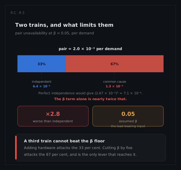
Two trains treated as independent would give
Fpair(independent) = (2.67 × 10⁻²)² = 7.1 × 10⁻⁴
They are not independent. Both trains share a design, a maintenance organisation, a fuel supply, a set of procedures and an ambient environment, and the standard way to represent that is the beta factor: a fraction β of each train's failure probability is attributed to causes that would fail both. With β = 0.05 the pair separates into two terms:
independent part = (0.95 × 2.67 × 10⁻²)² = 6.4 × 10⁻⁴
common-cause part = 0.05 × 2.67 × 10⁻² = 1.3 × 10⁻³
With a common-cause fraction β = 0.05 applied to the whole train unreliability, the realistic pair value is 2.0 × 10⁻³, and the common-cause term is roughly twice the independent one. The safety page works that split in full.
The common-cause term is roughly twice the independent one, and the honest pair value is 2.8 times worse than multiplication promised. The engineering reading is unambiguous: a third identical diesel would attack the 6.4 × 10⁻⁴ and leave the 1.3 × 10⁻³ untouched. Difference buys more than duplication. Diverse fuel supplies, staggered maintenance so one crew never works both trains in the same shift, physical separation and different procedures all attack β itself, which is the only term that matters once β is admitted. The safety page works the consequence side, where this unavailability enters a plant-level risk model rather than standing alone.
The surveillance paradox
The monthly start is what makes all of the above measurable, and it is not free. Between tests the train accumulates dangerous undetected failures, and each test both reveals them and takes the train out of service for two hours while it runs. Shortening the interval cuts the latent term and raises the test-induced term; there is an optimum, and practice does not chase it, because the surveillance start wears the machine and the crew running it accumulates dose. The testability page works that trade with the numbers.
What the analysis tells the engineer to do
Buy difference, not another diesel. A third identical train cubes the independent part, (0.95 × 2.67 × 10⁻²)³ = 1.63 × 10⁻⁵, and leaves the common-cause part alone: 1.35 × 10⁻³, a factor of 1.5 on 2.0 × 10⁻³ for a machine and a building. Driving β from 0.05 to 0.01 gives 9.7 × 10⁻⁴ from the two trains already installed, a factor of 2.1, and buys it with diverse fuel, staggered crews, separation and dissimilar starting arrangements.
Attack the run term, not only the start. Over the mission the run term of 2.37 × 10⁻² is 7.9 times the start term, and just under half of it is the support systems. Halve the fuel oil system's 250 per 10⁶ hours: the support total falls to 365, the train to 2.38 × 10⁻² and the pair to 1.7 × 10⁻³, a 15% improvement bought with fuel treatment rather than rotating machinery.
Stop buying demands and start buying evidence about β. Running the pair at the 4.4 × 10⁻³ bound moves it to 2.1 × 10⁻³; taking β from 0.05 to 0.10 moves it to 3.25 × 10⁻³. The 1,500 further train-years that would tighten the bound to 3.65 × 10⁻³ move the bounded pair to 2.04 × 10⁻³, a 3% correction to the term the answer is least sensitive to, while β has no demands behind it at all. Common-cause event reviews and audits of maintenance staggering are the cheaper evidence.
Keep the two clocks apart where the number is used. The start term is half the answer at three hours and a fiftieth over a week, so a single MTBF fitted at 24 hours is wrong at every other duration, and the plant model treats that duration as a distribution rather than a number.
What a different technique would have given
Predicting this machine from a handbook rather than measuring it would have produced a plausible per-hour rate and no per-demand term at all, because handbooks describe operating equipment and this machine spends its life not operating. The programme would then have had no way to represent the failure mode the whole risk model turns on, which is that the diesel does not start, and no way to bound its own confidence. Where the demands exist, measurement beats prediction so decisively that the interesting question becomes how to accumulate demands cheaply, which is precisely what a surveillance programme is.