

A level crossing is a small system that teaches a large lesson, because it contains two populations that behave completely differently and would be badly served by the same model. Its electronics sit in a benign cabinet and fail at random. Its barrier drives lift a boom several hundred thousand times and wear out. Applying one distribution to both is a common modelling error, and this page is about not making it.
The technique, and why this one
A mixed model: constant failure rates for the electronics, and a Weibull distribution fitted to field data for the barrier drives. The crossing fleet has been in service long enough to have a return stream, so the mechanical items no longer need to be predicted; they can be measured. That is always the better trade when the data exists, and it is exactly the handover that FRACAS is built to enable.
| Item | Model | Parameters | Source |
|---|---|---|---|
| Vital processor pair (2oo2) | exponential | λ = 40 per 10⁶ h | prediction |
| Barrier drive unit | Weibull | β = 1.9, η = 42,000 h | fitted from 6 years of field returns |
| Axle counter | exponential | λ = 120 per 10⁶ h | prediction |
| Signal lamp unit | exponential | λ = 200 per 10⁶ h each, 4 fitted | prediction |
| Road loop detector | exponential | λ = 80 per 10⁶ h | prediction |
| Crossing power supply unit | exponential | λ = 300 per 10⁶ h | prediction |
Fitting the barrier drive
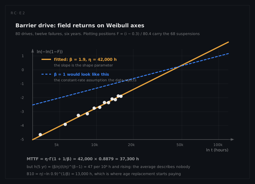
The data comes from 40 crossings, two drives each, over six years. Failure times are ranked and each is assigned a median rank estimate of the cumulative distribution using Bernard's approximation:
F̂(i) = (i − 0.3) / (n + 0.4)
With n = 80 drives in the fit, the first failure plots at F̂ = 0.7 / 80.4 = 0.0087 and the tenth at 9.7 / 80.4 = 0.121.
Plotting ln(t) against ln(−ln(1 − F̂)) linearises the Weibull, because taking logarithms twice of R(t) = e^(−(t/η)^β) gives
ln(−ln(1 − F(t))) = β·ln(t) − β·ln(η)
which is a straight line of slope β and intercept −β·ln η. The fitted line gives β = 1.9 and η = 42,000 hours. Suspensions matter here: most drives have not failed, and a fit that discarded them would be badly pessimistic, so the ranks are adjusted for the units still running.
What β = 1.9 changes
The mean life follows from the gamma function:
MTTF = η · Γ(1 + 1/β) = 42,000 × Γ(1.526) = 42,000 × 0.8874 = 37,300 h
Expressed as an average rate that is 10⁶ / 37,300 = 26.8 per 10⁶ hours. The design-stage book value used before the data arrived was 300 per 10⁶ hours per drive, a mean life of 10⁶ / 300 = 3,333 hours against the measured 37,300, so the prediction was pessimistic by a factor of 300 / 26.8 = 11.2. It would be tempting to conclude that the drives are simply better than expected and move on. That conclusion would miss the point entirely, because with β = 1.9 the average rate is not a usable description of anything.
The hazard rate is
h(t) = (β/η)·(t/η)^(β−1)
At five years in service (43,800 h) that is
h = (1.9 / 42,000) × (43,800 / 42,000)^0.9 = 4.52 × 10⁻⁵ × 1.039 = 4.7 × 10⁻⁵ per hour
or 47 per 10⁶ hours, and climbing. A drive that has been in service five years is nearly twice as likely to fail in the next hour as the fleet average suggests, and a drive installed last month is far less likely. The single number hides both facts. The testability page reads the same β as permission to monitor, because a hazard climbing this slowly has a physical ramp behind it that a motor-current signature can watch.
The survivor function says it in the currency a fleet manager uses:
R(t) = e^(−(t / 42,000)^1.9)
R(43,800) = e^(−(1.0429)^1.9) = e^(−1.083) = 0.339
A third of drives reach five years on their original installation, and the median drive lasts
B50 = η·(−ln 0.5)^(1/β) = 42,000 × (0.6931)^(1/1.9) = 42,000 × 0.8246 = 34,630 h
below the 37,300-hour mean, because a Weibull with β = 1.9 is skewed to the right.
The decision the shape makes possible
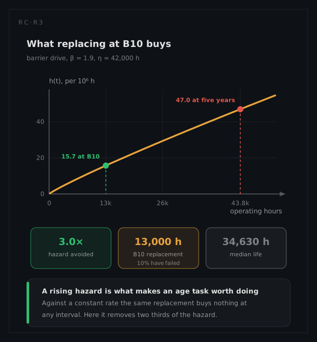
Here is the consequence that matters operationally, and it is a decision the exponential model can never justify. Because β > 1, preventive replacement works: a new drive really is better than an old one, so swapping a drive before it fails buys something. For an exponential item it buys nothing at all, because a survivor is statistically as good as new.
The B10 life, the age by which one drive in ten has failed, is
B10 = η·(−ln 0.9)^(1/β) = 42,000 × (0.10536)^(1/1.9) = 42,000 × 0.3059 = 12,850 h, taken as 13,000 h for the task
about eighteen months of continuous service. Replacing on an age basis somewhere between B10 and the characteristic life converts an unpredictable failure, which arrives during traffic and costs a possession at short notice, into a planned exchange during a scheduled possession. The maintainability page prices those two events against each other, and they are not close: the access constraint, not the repair, is what makes an unplanned drive failure expensive.
The age caps the hazard as well as the count:
h(13,000) = (1.9 / 42,000) × (13,000 / 42,000)^0.9 = 4.52 × 10⁻⁵ × 0.348 = 1.57 × 10⁻⁵ per hour
15.7 per 10⁶ hours, a third of the 47 a drive reaches by year five. Across the fleet, 80 drives running 80 × 8,760 = 700,800 drive-hours a year arrive at 700,800 / 37,300 = 18.8 failures a year under run-to-failure, against 700,800 / 13,000 = 53.9 age exchanges of which one in ten is a failure. That is 5.4 unplanned events instead of 18.8, bought with 48 extra planned ones that ride possessions already booked, and the availability page is where the possession is priced.
The rest of the crossing
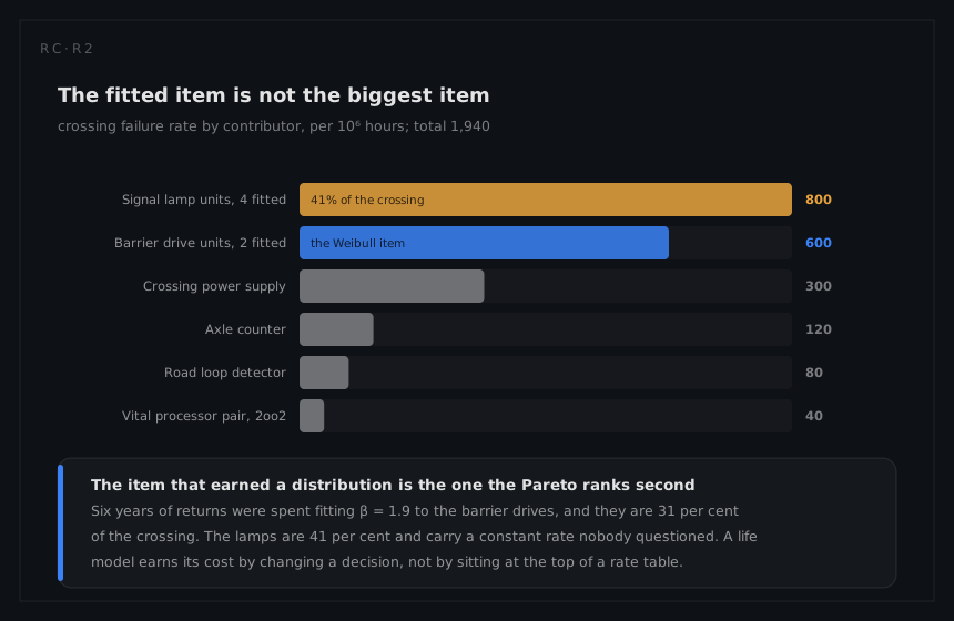
The electronics keep their constant rates, correctly. A vital processor pair, an axle counter and a loop detector have no wear mechanism that will express itself within the equipment's service life, and there is no field evidence of a rising hazard in the returns. Summed as a series chain with the drives carried at their design-stage book value, the whole crossing runs at 1,940 per 10⁶ hours, about 17 failures per crossing-year, and roughly 680 events a year across the 40-crossing fleet. The roll-up is a parts count and nothing cleverer:
| Item | λ (per 10⁶ h) | Contribution |
|---|---|---|
| Vital processor pair (2oo2) | 40 | 40 |
| Barrier drive unit, 2 fitted | 300 each | 600 |
| Axle counter | 120 | 120 |
| Signal lamp unit, 4 fitted | 200 each | 800 |
| Road loop detector | 80 | 80 |
| Crossing power supply unit | 300 | 300 |
| Crossing total | 1,940 |
Every other column then argues with that total. The availability page refuses it as an outage rate and backs out 192 per 10⁶ hours, a tenth of it; the testability page keeps all of it as a coverage denominator and gets 78 per cent.
A rate is not a survival probability, though, and over the 90-day proof-test interval of 2,160 hours the crossing's series product is worth writing out term by term:
Relec = e^(−2,160 × 40e-6) × e^(−2,160 × 120e-6) × e^(−2,160 × 800e-6) × e^(−2,160 × 80e-6) × e^(−2,160 × 300e-6)
= 0.9172 × 0.7717 × 0.1777 × 0.8413 × 0.5231 = 0.0553
Rdrives = (e^(−(2,160 / 42,000)^1.9))² = 0.9965² = 0.9929
giving 0.0553 × 0.9929 = 0.0549 for the quarter. The item that deserves the careful distribution is not the item that dominates the short-horizon answer: four lamp units take the product to 0.1777 on their own, and two new drives cost seven parts in a thousand.
The split in that table is the lesson the chapter exists to teach, and it runs both ways. The drive earns a Weibull because it has a wear mechanism, a duty that accumulates damage rather than elapsed time, and a return stream big enough for two parameters. The cabinet electronics earn a constant rate for the mirror-image reasons, and the storage array page defends that choice at length: screened parts, a controlled environment, and a service life shorter than the onset of any wear-out mechanism. Fitting a Weibull there returns β near 1 and spends a parameter to learn nothing. The error is not picking one model; it is picking once, for a whole system.
The failure-direction split is the other half of this system's story and belongs to safety rather than reliability: of that 1,940 only 6 per 10⁶ hours are failures that could show the crossing clear to road traffic with a train approaching, because the vital architecture is built to fail the other way. The safety page works that argument and the tolerable hazard rate behind it.
What the analysis tells the engineer to do
Write an age-replacement task for the barrier drives at 13,000 hours. It is defensible only because β = 1.9, and it buys two things that can be counted: each drive's hazard stays at or below 15.7 per 10⁶ hours instead of reaching 47 by year five, and the fleet's 18.8 unplanned drive failures a year become 5.4. An exponential model would have shown the two options as identical.
Re-baseline the spares forecast on the fit. At the book value the fleet's 700,800 drive-hours demand 700,800 × 300 × 10⁻⁶ = 210 replacement drives a year; at the fitted average they demand 18.8, and under age replacement 54. Ordering on the design-stage figure over-provisions elevenfold, and the same correction belongs in the prediction library before that value is reused on the next crossing design.
Pair the two drives on one visit whenever either falls due. The maintainability page shows 55 minutes paid once per visit against 95 minutes paid per drive, so the second drive costs 63 per cent of the first and no extra access delay. Retiring one drive before its own B10 is a small loss against the shape; saving a possession is not.
Spend the detection budget on the lamp units, not the drives. The 90-day product puts four lamp units at 0.1777 against 0.9929 for a new pair of drives, and the testability page reaches the same ranking from the other end, with 236 of the 426.8 per 10⁶ hours of undetected rate in that one population. Fitting the drive changed the maintenance policy; it did not change where the failures are.
What a different technique would have given
Keeping the drives exponential at the fitted average of 26.8 per 10⁶ hours would produce a crossing total near 1,395 rather than 1,940, would predict a flat arrival of drive failures across the fleet's age profile, and, worst of all, would say that preventive replacement is a waste of money. The fleet would then discover the rising hazard the expensive way, as a cluster of failures in the oldest installations that the model insisted should be spread evenly. The distribution is not a statistical nicety here; it is the difference between a maintenance policy that works and one that cannot.