

A level crossing sits on the network's critical path and can only be worked on when no trains are running. Almost everything distinctive about its availability follows from that one sentence: the technician can be ready, the van can be loaded and the fault can be understood, and the crossing still stays out of service until the night possession opens. Forty of these crossings make up the reference fleet, each running continuously, 8,760 hours a year.
The crossing is also the page where the two ledgers must be kept apart. The reliability column counts failures; the availability column counts outages; and on this system the two populations differ by a factor of ten. A programme that quietly swaps one for the other will produce an availability forecast wrong by an order of magnitude, in whichever direction suits the author.
The technique, and why this one
Steady-state availability arithmetic on a series reliability block diagram, computed in unavailability currency (q = λ × MDT), with the possession wait carried as administrative delay rather than repair. The crossing earns the closed form honestly. There is no redundancy worth modelling, so no repair coupling; there is one crew per event, so no queue; the items are independent; and detection is immediate for everything that matters, because a crossing that has failed announces itself by stopping trains. That is the complete list of conditions under which the product rule is legitimate, and when they hold, a state model or a simulation adds cost and no accuracy.
| Item | Availability model | λ (per 10⁶ h) | Contributes to the outage ledger? |
|---|---|---|---|
| Vital processor pair (2oo2) | exponential, fails to the safe side | 40 | Yes: the crossing goes to its protective state and trains stop |
| Barrier drive unit (2 fitted) | Weibull in service (β = 1.9, η = 42,000 h), constant rate in the ledger | 300 each | In part: only a drive that fails to lower stops trains |
| Axle counter | exponential | 120 | In part: many faults clear on a reset |
| Signal lamp unit (4 fitted) | exponential, redundant set | 200 each | No: four lamps are fitted |
| Road loop detector | exponential | 80 | No: the crossing degrades rather than stops |
| Crossing power supply | exponential, battery-backed | 300 | Yes on total loss |
| Access | administrative delay | night possession only | 7 h added to every event |
Two ledgers, one crossing
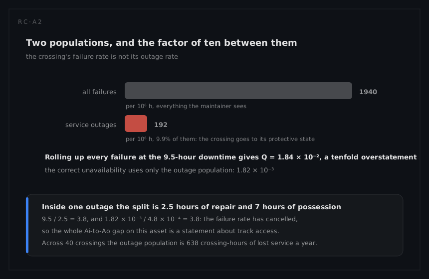
Start with the calculation an unwary analyst produces, precisely so that it can be rejected. The crossing's total failure rate is 1,940 per 10⁶ hours, mean downtime including the possession wait is 9.5 hours, and the series roll-up in unavailability currency is
Q = Σλᵢ × MDT = 1,940 × 10⁻⁶ × 9.5 = 1.84 × 10⁻²
A = 1 − 1.84 × 10⁻² = 0.9816
The crossing actually reports Ao = 0.99818. The naive roll-up is wrong by a factor of ten in unavailability, and no amount of care with the arithmetic will fix it, because the error is in the population, not the sum. Of the 1,940 per 10⁶ hours the equipment produces, most events do not take the crossing out of service: one lamp of four fails and three remain lit, an axle counter throws a fault that clears on a reset, a road loop degrades into a fallback detection mode, a barrier fails in the down position and inconveniences road traffic while trains run normally.
Back the service-affecting rate out of the reported inherent availability, which is the honest way to obtain it, because the mapping from failures to outages is an engineering judgement recorded in the ledger and not a sum of a rate table:
qi = 1 − 0.99952 = 4.8 × 10⁻⁴
λoutage = qi / MTTR = 4.8 × 10⁻⁴ / 2.5 = 1.92 × 10⁻⁴ = 192 per 10⁶ h
That is 9.9% of the crossing's total failure rate, and it is the only rate the availability model is entitled to use. The reliability ledger and the availability ledger count different things, and the ratio between them is a design property, not a rounding error. Publish the outage definition with the number, or the number means whatever its author needed it to mean.
The possession, priced
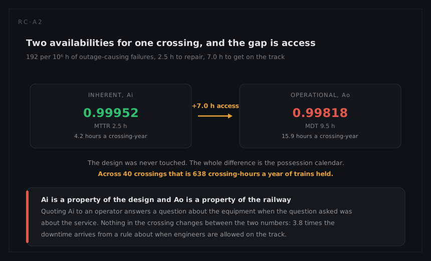
With the service-affecting rate established, both availabilities fall out of the same formula with different downtimes in it.
qi = λoutage × MTTR = 192 × 10⁻⁶ × 2.5 = 4.8 × 10⁻⁴ → Ai = 0.99952
qo = λoutage × MDT = 192 × 10⁻⁶ × 9.5 = 1.82 × 10⁻³ → Ao = 0.99818
In hours, over a continuous year:
inherent downtime = 4.8 × 10⁻⁴ × 8,760 = 4.2 hours per crossing-year
operational downtime = 1.82 × 10⁻³ × 8,760 = 15.9 hours per crossing-year
fleet exposure = 1.82 × 10⁻³ × 8,760 × 40 = 638 crossing-hours a year
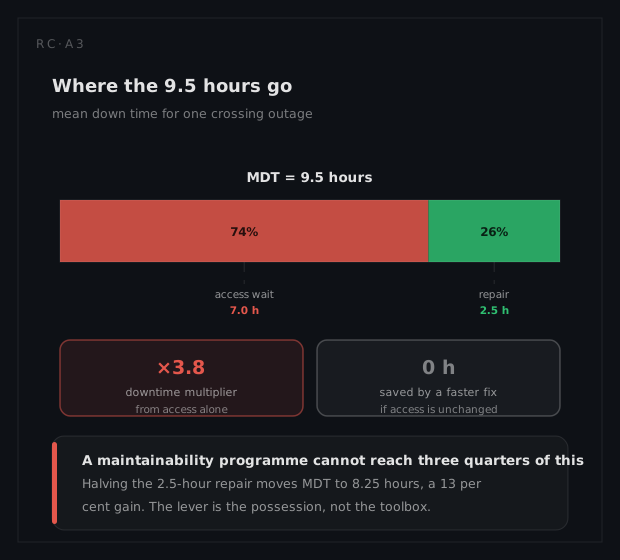
The gap is 11.7 hours a crossing-year across about 1.68 outage events (192 × 10⁻⁶ × 8,760), which is seven hours of waiting per event, and seven hours is exactly the difference between the 2.5-hour active repair and the 9.5-hour mean downtime. Notice what has happened to the failure rate: 9.5 divided by 2.5 is 3.8, and 1.82 × 10⁻³ divided by 4.8 × 10⁻⁴ is also 3.8. When the same events are counted in both ledgers, the ratio of the two availabilities is nothing more than the ratio of the two downtimes, and an Ai-to-Ao gap can therefore always be read directly as a statement about delay, never needing a reliability argument to explain it.
The barrier drive makes the number move
One item on the list is not exponential, and its behaviour puts a slow drift under everything above. The reliability page fits the barrier drives from six years of field returns and obtains β = 1.9, η = 42,000 hours, which is a clear wear-out signature. The average rate implied by that fit is
MTTF = η · Γ(1 + 1/β) = 42,000 × Γ(1.526) = 42,000 × 0.8874 = 37,270 h, quoted as 37,300 h
or 26.8 per 10⁶ hours, but the instantaneous hazard at five years in service (43,800 h) is
h(t) = (β/η)(t/η)^(β−1) = (1.9 / 42,000) × (43,800 / 42,000)^0.9 = 4.7 × 10⁻⁵ per hour
which is 47 per 10⁶ hours and rising. An availability model built on a constant rate is therefore quoting a number that is optimistic for old installations and pessimistic for new ones, and the fleet average will drift downward as the installed base ages. The availability consequence of β > 1 is the same one the reliability page draws and it is worth repeating in this currency: because a new drive really is better than an old one, age replacement converts an unplanned outage into a planned exchange inside a possession that was going to happen anyway, and on this system a planned exchange costs approximately nothing while an unplanned one costs 9.5 hours. Replacing at
B10 = η(−ln 0.9)^(1/β) = 42,000 × (0.10536)^(1/1.9) = 42,000 × 0.3059 = 12,850 h, taken as 13,000 h for the task
puts nine drives in ten into the free column.
What the analysis tells the engineer to do
Seven of every 9.5 hours are access, so the availability plan for this crossing is an access plan. Three interventions attack it and none of them is a spare part. Batch the work so that one possession clears several faults, which is maintenance task analysis applied to a possession window rather than to a single job. Improve remote diagnosis so that the right part travels on the first visit, because a wrong part costs a whole extra possession cycle rather than a whole extra van journey; the testability page works the 78% remote-monitoring coverage that decides this. And at design time, position as much equipment as possible where it can be reached without a possession at all, which is the one intervention that removes the seven hours instead of amortising them.
Buying stock, by contrast, does nothing measurable here. That is the opposite conclusion to the aircraft in this column, whose entire gap was a spare in the wrong place, and the two systems reached it with identical arithmetic. The formula does not tell you where the downtime is; the ledger does.
What a different technique would have given
The plausible alternative is a Monte Carlo model of the possession calendar. Possessions are granted on a fixed rota, so the wait is not a smooth mean of seven hours but a hard structure: a fault at 06:00 waits sixteen hours and a fault at 22:00 waits none. A simulation would sample the fault time uniformly across the day, apply the rota, and produce the full distribution of restoration times instead of its average.
It would have produced the same 638 crossing-hours, because the mean of a distribution is the mean whichever way it is obtained, and the fleet ledger is built on means. It was rejected on that basis: do not simulate what you can integrate. The rejection is conditional rather than permanent, though, and it is worth knowing when it flips. The moment the question becomes contractual, as in "what percentage of crossing faults are cleared within 24 hours", the mean is useless and the closed form has nothing to offer, because that is a question about the tail of the possession-wait distribution. Change the question and the right technique changes with it.