

A wayside level-crossing controller: a 2oo2 vital processor, two barrier drive units, an axle counter, four road-signal lamp units and a road-loop detector, running continuously across a reference fleet of forty crossings. The technician reaches the roadside quickly and finishes the work in two and a half hours. The crossing is nevertheless out of service for nine and a half, and nothing the design does to the repair will change that.
This is the chapter's sharpest case of a distinction maintainability engineers spend careers explaining: repair time and downtime are different quantities, owned by different people, fixed with different budgets. Here they differ by a factor of nearly four and the larger is not a design property at all. What makes the crossing worth a page is that once the access constraint is admitted, the engineering does not stop; it moves.
The technique, and why this one
An elemental task build-up for the dominant corrective action, placed inside an additive downtime model that separates active repair from access delay, with the repair time treated as a lognormal so the fixed possession window can be scored as a percentile rather than a mean. The first two parts are ordinary bookkeeping. The third earns its keep, because the possession is a hard boundary: a job that runs long does not finish late, it finishes tomorrow, and only a distribution says how often.
| Quantity | Model used | Value |
|---|---|---|
| Barrier drive replacement | elemental task build-up, eight elements | 2.5 h active |
| Spread of the active repair | lognormal, σ = 0.7 as the chapter's canonical spread | tmed = 1.96 h |
| Access wait | deterministic delay, set by the possession calendar | 7.0 h |
| Mean downtime | additive: active plus access | 9.5 h |
| Service-affecting failure rate | inferred from the availability figures | 192 per 10⁶ h |
| Barrier drive life | Weibull fitted from six years of field returns | β = 1.9, η = 42,000 h |
The Weibull row is borrowed rather than derived: it is fitted on the reliability page and appears here only because it decides whether preventive replacement is worth planning into a possession.
Building the drive replacement from its elements
| Element | Time (min) | What sets it |
|---|---|---|
| Preparation and safety isolation | 20 | possession protection, lock-out, documentation |
| Fault localization | 10 | condition monitoring has usually narrowed it |
| Fault isolation | 10 | drive-side or control-side |
| Disassembly and access | 15 | cabinet and drive housing |
| Interchange | 45 | drive removal and refit, boom disconnection |
| Reassembly | 15 | housing and cabinet closed |
| Alignment and calibration | 25 | boom travel, limit switches, proving switch |
| Checkout | 10 | full sequence test with the signalling interface |
| Total | 150 (2.5 h) |
Two elements stand out against the aircraft's profile on the defence and aerospace page. Alignment is 25 minutes and 17% of the job where the aircraft's LRUs needed none, because a barrier boom's travel and limit positions must be re-established every time. Preparation is 20 minutes because it includes safety isolation on a live railway, paid on every job whatever is replaced. Both facts matter below.
The downtime quoted, and the downtime delivered
The specification's 9.5 hours is 2.5 hours of work plus 7.0 hours waiting for the night possession, so active repair is 26% of downtime. Halving the active repair through better modularity and sharper diagnostics, a substantial redesign of the wayside cabinet, takes 9.5 hours to 8.25: an improvement of 13%. Every hour bought on the access side is worth the same as an hour bought on the wrench side, and seven of them are lying untouched on the access side. This is the MTTR-versus-MDT trap in its purest available form.
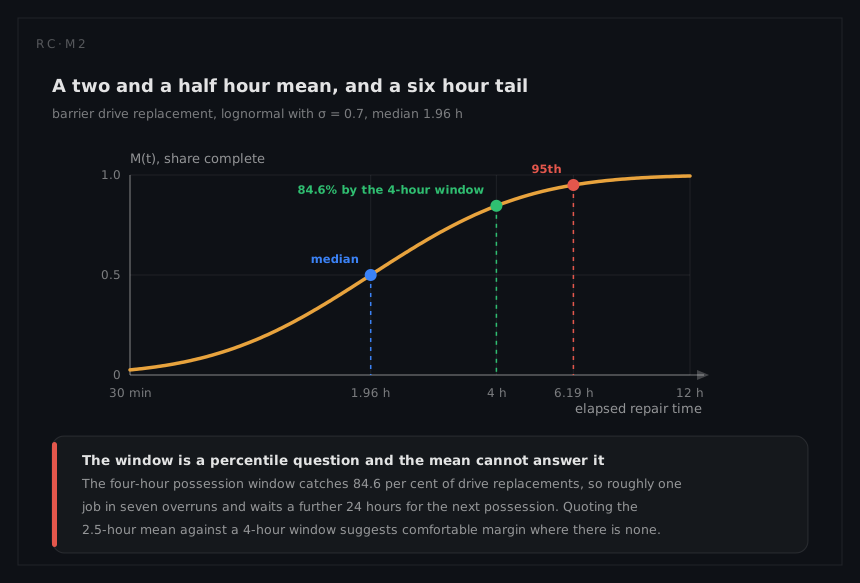
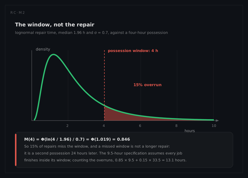
The 9.5 hours also assumes something it never states: that every job finishes inside its window. Treat the active repair as lognormal with mean 2.5 hours and σ = 0.7, so
tmed = 2.5 / e^(0.7²/2) = 2.5 / 1.2776 = 1.96 h
Take the working window inside a night possession as four hours once travel, safety setup and hand-back are deducted; that is a planning figure rather than a specification value, but it is the right order. Then
M(4) = Φ(ln(4 / 1.96) / 0.7) = Φ(0.713 / 0.7) = Φ(1.019) = 0.846
and about one job in seven does not finish. The percentiles agree:
t₀.90 = 1.96 × e^(1.282 × 0.7) = 1.96 × 2.452 = 4.80 h
t₀.95 = 1.96 × e^(1.645 × 0.7) = 1.96 × 3.163 = 6.19 h
The 90th-percentile job needs 4.8 hours and the window offers 4. An overrun is not a late finish: the crossing is handed back in its fail-safe state and the work resumes at the next possession, 24 hours away.
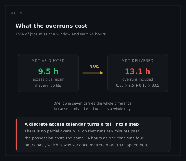
MDTeffective = 0.85 × 9.5 + 0.15 × (9.5 + 24) = 8.08 + 5.03 = 13.1 h
The specification's 9.5-hour mean downtime is 13.1 hours once window overruns are counted, and the whole difference comes from the spread rather than the mean. A change that left the 2.5-hour mean alone but cut σ from 0.7 to 0.4 moves the median to 2.5 / e^0.08 = 2.31 h and raises M(4) to Φ(ln(4 / 2.31) / 0.4) = Φ(1.375) = 0.915, roughly halving overruns from 15% to about 8.5%. Predictability here is worth more than speed.
Which failures actually take the crossing out of service
The crossing's total rate is 1,940 per 10⁶ hours, and it is tempting to multiply that by the downtime. The availability figures refuse to agree and are the better witness. From inherent availability,
Ui = 1 − 0.99952 = 4.8 × 10⁻⁴ = λeff × 2.5 h → λeff = 1.92 × 10⁻⁴ per hour
and from operational availability,
Uo = 1 − 0.99818 = 1.82 × 10⁻³ = λeff × 9.5 h → λeff = 1.92 × 10⁻⁴ per hour
The two agree to three figures at 192 per 10⁶ hours, a tenth of the crossing's total. Nine failures in ten do not take the crossing out of service, because four lamp units and two barrier drives carry redundancy and because many failures are right-side failures that leave the barriers down: safe, and costing road delay rather than availability. The safety page works the direction of failure. For maintainability the consequence is procedural: the work-order stream and the downtime-driving stream differ by a factor of ten, so a technician's job count is not an availability input.
Across the fleet, (1 − 0.99818) × 8,760 × 40 = 638 crossing-hours of degraded operation a year. At the 13.1-hour effective downtime, 1.92 × 10⁻⁴ × 13.1 = 2.51 × 10⁻³ and the fleet total rises to 879 crossing-hours: 240 crossing-hours a year purchased by the tail of a repair-time distribution.
What the analysis tells the engineer to do
If access is the scarce resource, the objective stops being minutes per repair and becomes work completed per possession, which changes three decisions at once.
It makes preventive replacement worth planning. With β = 1.9 the drives genuinely age, so a new drive is better than an old one, and the B10 life of 13,000 hours computed on the reliability page becomes a schedulable date. Age replacement converts a failure arriving during traffic into an exchange during a possession that was going to be booked anyway: a straight RCM argument, with operational delay as the consequence class and scheduled restoration as the applicable task.
It makes the second job on a visit nearly free. From the element table, 55 minutes of preparation, localization, isolation and access are paid once per visit while 95 minutes of interchange, reassembly, alignment and checkout are paid per drive. Both drives on one visit cost 55 + 190 = 245 minutes rather than 300, so the second drive costs 63% of the first and consumes no extra access delay. That 245 minutes also exceeds the four-hour window, which is the kind of finding a task analysis exists for and never appears in an MTTR figure.
And it re-prices condition monitoring. Remote monitoring detects 78% of the failure rate and makes no repair faster. What it does is put the job on the possession plan before the possession is booked, which is worth the entire 7-hour access delay. No roadside diagnostic improvement could return that much.
What a different technique would have given
The conventional treatment specifies a mean active repair time and stops. It produces 2.5 hours, is met by the design, and is silent on everything this page found: it cannot say that 15% of jobs overrun their window, cannot show that the true mean downtime is 13.1 rather than 9.5 hours, and cannot value a variance reduction that never touches the mean it reports. A programme holding a satisfied 2.5-hour requirement would have no reason to fund the change that matters most.
Modelling the repair as exponential would at least produce a distribution, but the wrong one. With mean 2.5 hours, M(4) = 1 − e^(−4 / 2.5) = 0.798, forecasting a 20% overrun rate against the lognormal's 15%, and putting the median at 2.5 × ln 2 = 1.73 hours against the fitted 1.96. Its convenience is real and belongs in the availability algebra where only means survive. Its shape is not the shape of repair work, and on a system governed by a hard window the shape is the whole question.