

A wayside level crossing is watched from a control centre miles away and touched by human hands only during a night possession of the railway. That single operational fact reshapes the testability question. On an aircraft, detection buys a faster turnround; here it buys the right to book the possession at all, because a technician who arrives without knowing what failed has spent the only access window the railway will grant for a fortnight.
There is a second question hiding underneath the first, and it is the more serious one. The crossing contains a proving switch that confirms the barrier is physically down. It contributes almost nothing to the failure rate and everything to the safety case, and no amount of rate-weighted thinking will find it. This page works both: the coverage arithmetic that decides the maintenance economics, and the failure-finding interval that decides whether the SIL 4 argument stands up.
The technique, and why this one
Rate-weighted fault detection rate computed over the mode inventory, plus an RCM failure-finding interval sized from a latent-unavailability allowance rather than from a maintenance calendar. Two techniques because the crossing has two testability problems with different currencies: the announced-failure population is priced in possessions, and the latent population is priced in probability of failure on demand. Using one method for both is the classic error, and it always sacrifices the switch.
| Item | λ per 10⁶ h | Model used | Test means credited |
|---|---|---|---|
| Vital processor pair (2oo2) | 40 | constant λ; fails to the safe side by design | continuous self-test and 2oo2 disagreement |
| Barrier drive unit (each, 2) | 600 total | Weibull, β = 1.9, η = 42,000 h, fitted from six years of field returns | motor current signature and barrier travel timing |
| Axle counter | 120 | constant λ | count integrity and reset diagnostics |
| Signal lamp unit (each, 4) | 800 total | constant λ | lamp current monitoring per unit |
| Road loop detector | 80 | constant λ | loop inductance plausibility |
| Crossing power supply unit | 300 | constant λ | supply voltage and battery state |
| Barrier-down proving switch | 0.9 dangerous undetected | constant λ, dormant | nothing continuous: proof test only |
The barrier drive is the reason a mixed model is compulsory. It lifts a boom several hundred thousand times and wears; its electronics neighbours sit in a benign cabinet and do not. The Weibull parameters come from the reliability page, which fits them, and they matter here for a reason that page does not need: a rising hazard means degradation precedes failure, and degradation is something a monitor can watch.
Rolling up what the monitoring sees
FDR = Σλ(detected) / Σλ(all)
| Item | λ per 10⁶ h | Detected | Undetected λ |
|---|---|---|---|
| Vital processor pair | 40 | 95.0% | 2.0 |
| Barrier drives (2) | 600 | 85.0% | 90.0 |
| Axle counter | 120 | 88.0% | 14.4 |
| Signal lamp units (4) | 800 | 70.5% | 236.0 |
| Road loop detector | 80 | 62.0% | 30.4 |
| Crossing power supply | 300 | 82.0% | 54.0 |
| Total | 1,940 | 426.8 |
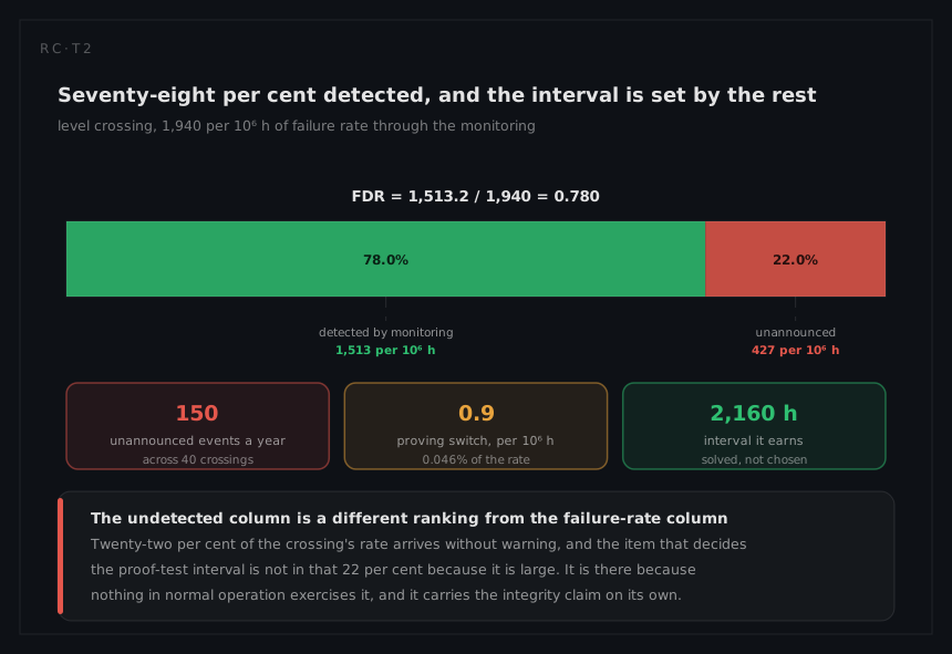
FDR = (1,940 − 426.8) / 1,940 = 1,513.2 / 1,940 = 0.780
Seventy-eight per cent is the lowest headline coverage in this chapter and it is not a failure of engineering ambition. The undetected column says why: 236 of the 426.8 sits in the signal lamps, not because lamps are hard to monitor but because there are four of them at 200 per 10⁶ hours each, and current monitoring catches an open filament far more reliably than it catches a dim, misaimed or partially obscured lamp. The largest blind spot in the system is the item with the most copies and the crudest sensor, which is the general shape of an undetected-λ Pareto and almost never the shape of the failure-rate Pareto.
In annual terms, at 8,760 hours a year across the 40-crossing fleet:
unannounced events per year = 426.8 × 10⁻⁶ × 8,760 × 40 = 150
against roughly 680 events in total. One hundred and fifty times a year, somebody finds out from a road user, a driver or a routine visit. Each of those is a possession booked without a diagnosis, which is why 78% is worth paying to improve even though it looks unimpressive beside a satellite's 96%. The maintainability page prices the difference: active repair is 2.5 hours inside a mean down time of 9.5 hours, and the gap is access, not diagnosis, so a wasted possession is the expensive event.
Sizing the interval on the item that carries no rate
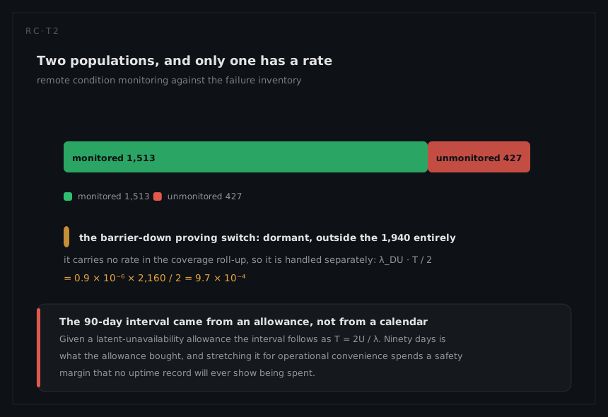
The proving switch is 0.9 per 10⁶ hours of dangerous undetected failure, which is 0.046% of the crossing's total. A coverage budget allocated by λ would place it last and would be correct by its own logic. It is also the item whose silent failure lets the crossing report itself proven when it is not, and the safety page shows the SIL 4 argument, tolerable hazard rate 10⁻⁹ per hour, collapsing without it.
The remedy is a failure-finding task, and the interval is computable rather than conventional. Average latent unavailability of a dormant item proof-tested every T hours is
Ulatent = λDU × T / 2
Invert it against an allowance. If the safety case allocates 1.0 × 10⁻³ of latent unavailability to this switch:
T = 2 × Uallowed / λDU = 2 × 1.0 × 10⁻³ / (0.9 × 10⁻⁶) = 2,222 h = 93 days
which is where the 90-day interval comes from. Checking the achieved value at the interval actually adopted, T = 2,160 hours:
Ulatent = 0.9 × 10⁻⁶ × 2,160 / 2 = 9.7 × 10⁻⁴
just inside the allowance. Move to a 30-day cycle and the same arithmetic gives 0.9 × 10⁻⁶ × 720 / 2 = 3.2 × 10⁻⁴, a threefold improvement bought entirely with scheduling. The point is not the specific number but the direction of the derivation: the allowance sets the interval, the interval does not set the allowance.
Why a rising hazard makes the drive monitorable
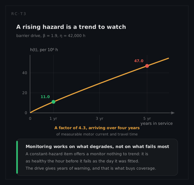
The barrier drive's β = 1.9 does something for testability that no exponential item offers. The hazard rate
h(t) = (β/η)·(t/η)^(β−1)
evaluated at one year and at five years in service gives
h(8,760) = (1.9/42,000) × (8,760/42,000)^0.9 = 4.52 × 10⁻⁵ × 0.244 = 1.10 × 10⁻⁵ per hour
h(43,800) = (1.9/42,000) × (43,800/42,000)^0.9 = 4.52 × 10⁻⁵ × 1.039 = 4.70 × 10⁻⁵ per hour
11.0 per 10⁶ hours rising to 47, a factor of 4.3 across four years. A hazard that climbs that slowly and that steadily is a hazard with a physical ramp behind it: bearing friction, gearbox backlash, seal drag, all of which show up as drive-motor current and barrier travel time long before the boom fails to lift. The monitor is therefore not a failure detector at all, it is a degradation detector, and that is only available because the item wears. For a genuinely exponential item there is nothing to see coming, and a monitor can only report the event after it has happened. The 85% credited to the drives in the table above is achievable for exactly this reason.
What the analysis tells you to do
The lamp units own the undetected budget, so that is where the coverage money goes: a photometric check rather than a current check converts a large share of 236 per 10⁶ hours and is a sensor change, not an architecture change. The proving switch owns the safety argument, so its interval is fixed by the allowance and defended against every attempt to fold it into a convenient annual visit. The barrier drives justify a trend rather than a threshold: with four years of warning available, a drive replacement can go into a possession already booked for something else, and B10 = 13,000 hours gives the age at which that becomes worth scheduling. Detection, interval and preventive replacement are three different answers, and the mode list decides which each item gets.
What a different technique would have given
The common alternative is to set the proving-switch check by maintenance convention: fold it into the annual visit, because that is when somebody is on site anyway. The arithmetic is unforgiving:
Ulatent = 0.9 × 10⁻⁶ × 8,760 / 2 = 3.9 × 10⁻³
four times the allowance, from a decision nobody would recognise as a safety decision when they made it. Stretch it to a four-yearly overhaul and it becomes 0.9 × 10⁻⁶ × 35,040 / 2 = 1.6 × 10⁻², sixteen times over. A second alternative is milder and more common: quote coverage by counting items rather than weighting by rate. The unweighted mean of the six item coverages above is 80.4% against the weighted 78.0%, a difference small enough to look like rounding, which is precisely why it is dangerous. It treats the 40 per 10⁶ hour processor and the 800 per 10⁶ hour lamp population as equals, and a team optimising the counted number would work on the processor. The weighting is not a refinement; it is what makes the number predict the fleet's experience.