

The same aircraft electrical system, and the same FMECA worksheet that the safety page built. Safety read that worksheet for consequence and produced a fault tree. This page reads the identical seventeen modes for a different question: which of them announces itself, how precisely, and how often the announcement is wrong. Three numbers come out, and the whole avionics maintenance economy rests on them.
The technique, and why this one
A dependency-matrix computation over the FMECA mode inventory, producing fault detection rate, fault isolation rate and false alarm rate. The choice is forced by timing rather than preference: these figures are contractual and have to be quoted years before hardware exists to demonstrate on. The only thing available at that point is the mode list, the design's monitors, and an honest statement of which monitor responds to which mode. That is a dependency matrix, and everything below is arithmetic on it.
Reusing the safety worksheet rather than building a second inventory is not a convenience. It is the control that keeps the two analyses honest: any mode the testability engineer cannot assign a detection means to is a mode the safety engineer has classified and is relying on, and the two disciplines discover their disagreements while the design is still soft.
Detection means are continuous BIT (CBIT), power-up BIT (PBIT), initiated BIT (IBIT), periodic functional check (FC) and not detected (ND).
| # | Mode | λ, all units, per 10⁶ FH | Detected by | Isolates to |
|---|---|---|---|---|
| 1 | IDG loss of output | 275.0 | CBIT | 1 LRU |
| 2 | IDG overvoltage | 50.0 | CBIT | 1 LRU |
| 3 | IDG degraded output | 100.0 | CBIT | 2 LRUs |
| 4 | IDG drive mechanical | 75.0 | 49.0 CBIT, 26.0 ND | 1 LRU |
| 5 | GCU fails to trip | 45.0 | IBIT | 1 LRU |
| 6 | GCU spurious trip | 81.0 | CBIT | 1 LRU |
| 7 | GCU loss of regulation | 36.0 | CBIT | 2 LRUs |
| 8 | GCU undetected internal fault | 18.0 | ND | n/a |
| 9 | Contactor fails open | 45.0 | CBIT | 3 LRUs |
| 10 | Contactor welded closed | 22.5 | IBIT | 3 LRUs |
| 11 | Contactor high resistance | 7.5 | ND | n/a |
| 12 | APU fails to start | 120.0 | PBIT | 1 LRU |
| 13 | APU loss of output | 135.0 | CBIT | 1 LRU |
| 14 | APU degraded output | 45.0 | CBIT | 2 LRUs |
| 15 | RAT fails to deploy | 26.0 | ND, FC at 500 FH | n/a |
| 16 | RAT deploys, no output | 10.0 | ND, FC at 500 FH | n/a |
| 17 | RAT spurious deploy | 4.0 | CBIT | 1 LRU |
| Total | 1,095.0 |
FDR: what the system sees
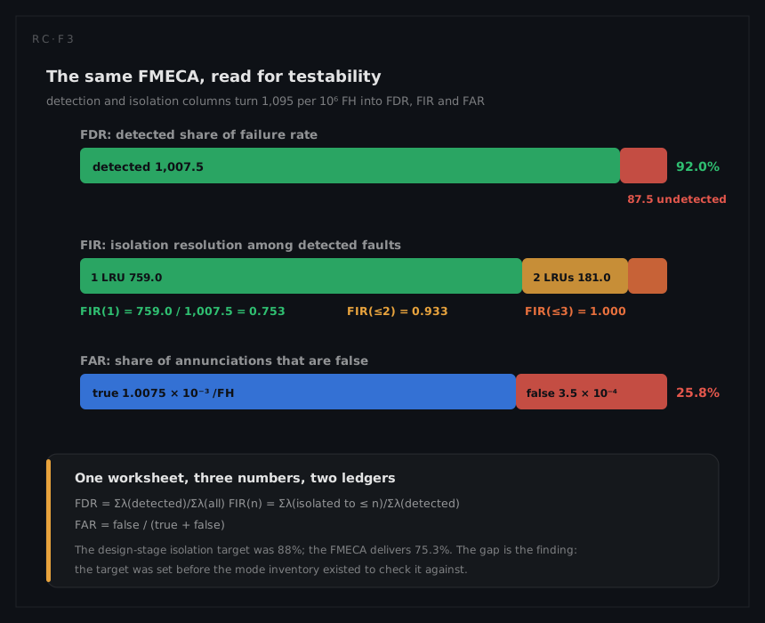
Fault detection rate is the failure-rate-weighted share of the inventory the test means respond to, never the share of modes:
FDR = Σλ(detected) / Σλ(all)
The undetected set is five entries: 26.0 of IDG drive degradation before it annunciates, 18.0 of GCU internal faults, 7.5 of contactor high resistance, and the two RAT modes at 26.0 and 10.0.
Σλ(undetected) = 26.0 + 18.0 + 7.5 + 26.0 + 10.0 = 87.5
FDR = (1,095.0 − 87.5) / 1,095.0 = 1,007.5 / 1,095.0 = 0.920
Ninety-two per cent, which is the figure quoted in the specification. Counted by mode instead, five undetected modes out of seventeen would read as 70.6% coverage, and neither number describes the other. The weighted figure is the one that predicts what the fleet experiences, for the reason the foundations chapter works through: the fleet meets modes in proportion to their rates.
FIR: how precisely it points
Fault isolation rate is computed over the detected population only, because a fault nobody saw cannot be isolated:
FIR(n) = Σλ(isolated to ≤ n units) / Σλ(detected)
Grouping the detected rows:
to 1 LRU: 275.0 + 50.0 + 49.0 + 45.0 + 81.0 + 120.0 + 135.0 + 4.0 = 759.0 to 2 LRUs: 100.0 + 36.0 + 45.0 = 181.0 to 3 LRUs: 45.0 + 22.5 = 67.5
which reconciles: 759.0 + 181.0 + 67.5 = 1,007.5. Then
FIR(1) = 759.0 / 1,007.5 = 0.753 FIR(≤2) = 940.0 / 1,007.5 = 0.933 FIR(≤3) = 1,007.5 / 1,007.5 = 1.000
The design-stage target was 88% isolation to a single unit and the mode inventory delivers 75.3%. That gap is the most useful output on this page, and it is not an error in either number: the target was written before an inventory existed to check it against, which is the normal sequence and the reason this analysis is run. Closing it means finding the modes in the 2-LRU and 3-LRU groups and giving them a discriminating test, and the worksheet says exactly where they are: the two degraded-output modes, the regulation mode and both contactor modes.
FAR: whether anyone believes it
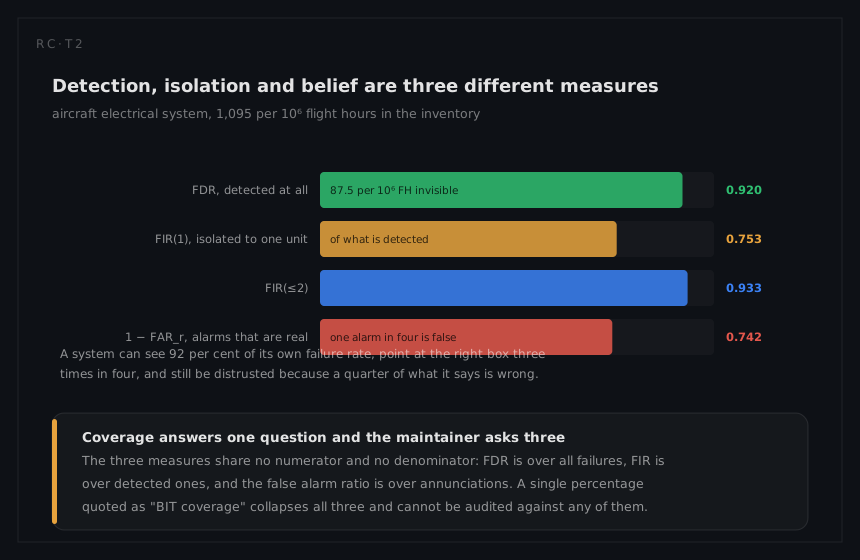
Detection and isolation are worthless if the crew has learned to ignore the annunciation, so the third number is the one that decides the value of the other two. Observed false indications run at 0.35 per 1,000 flight hours, while true annunciations arrive at the detected rate:
true rate = 1,007.5 × 10⁻⁶ = 1.0075 × 10⁻³ per FH false rate = 3.5 × 10⁻⁴ per FH
FARr = false / (true + false) = 3.5 × 10⁻⁴ / 1.3575 × 10⁻³ = 0.258
Two quantities share the name and only one of them is a rate. FARh = 3.5 × 10⁻⁴ per flight hour is what multiplies by fleet hours into a maintenance load; FARr = 0.258 is dimensionless and is what a crew experiences. A specification that says "false alarm rate shall not exceed 0.25" without saying which one has specified nothing, and the two move independently: improving detection raises the true rate, which lowers FARr while leaving FARh untouched.
One annunciation in four is false. That single figure explains behaviour that looks irrational from a design office: crews deferring on a caption, line technicians running a second test before believing the first, and a removal rate that exceeds the failure rate.
What it costs, in units pulled off the aircraft
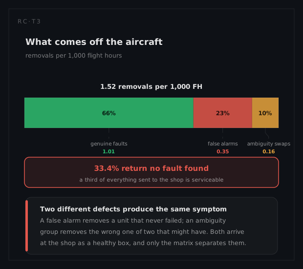
The three numbers combine into the quantity the support organisation actually feels. Per 1,000 flight hours:
true detected faults = 1.0075 false alarms = 0.35 ambiguity-driven extra removals = 0.181 × 0.5 + 0.0675 × 1.0 = 0.158
using the expected-swap result that a group of n needs (n+1)/2 attempts, so a 2-LRU group averages half an extra unit and a 3-LRU group one extra. Total removals are 1.0075 + 0.35 + 0.158 = 1.52 per 1,000 flight hours, of which 33.4% return no fault found. A third of everything this aircraft sends to the shop is serviceable.
The improvement agenda falls straight out and is ordered by what each fix buys. Attacking the false alarm rate removes 0.35 removals per 1,000 hours and, more importantly, restores the credibility the other numbers depend on. Attacking the ambiguity groups removes 0.158. Attacking the undetected 87.5 removes no removals at all and instead pays into a different ledger entirely: the RAT's 36 per 10⁶ hours of silent failure is the term that dominates the safety page's fault tree at 9.0 × 10⁻³, and halving the 500-hour check interval halves it.
That is the honest summary of this page. Coverage buys its value in three different ledgers: isolation in the maintenance cost that maintainability prices, false alarms in dispatch and in trust that availability prices, and the undetected fraction in the latent risk that safety prices. Optimising the headline percentage without asking which ledger the complement is filling is the standard way to improve a number and nothing else.
What a different technique would have given
Waiting for a demonstration instead of computing from the dependency matrix would have produced a defensible figure and produced it far too late. A fault-insertion campaign is the right way to verify these numbers, and it happens on hardware, near the end of the programme, when the discovery that isolation is 75% rather than 88% costs a redesign instead of a test point. Worse, an inserted-fault sample is drawn from the modes someone chose to insert, so a campaign that never inserts a slow IDG drive degradation will report a coverage the fleet will not reproduce. The dependency model is weaker evidence and vastly better timing, which is why the discipline computes first and demonstrates second rather than the other way round.