

Two engine-driven integrated drive generators, an auxiliary power unit generator, a ram air turbine, two generator control units and the contactors that tie the buses together. The question the programme has to answer is not how often a generator fails. It is how often the aeroplane loses all of its alternating-current sources at once, and the distance between those two questions is where the entire architecture lives.
The technique, and why this one
Part-stress prediction for the item rates, an RBD for the architecture, a fault tree for the top event. The choice of a constant failure rate here is deliberate and defensible: these are mature avionics assemblies operating in their useful life, screened to an aerospace parts standard, and at the point the analysis is needed no fleet exists to measure. When there is no data and the physics is dominated by randomly arriving stress rather than accumulating wear, the exponential model is the honest default rather than a lazy one. The rates carry their own conservatism: MIL-HDBK-217F part models are point estimates, not bounds, so the conservatism below has to be argued item by item rather than assumed.
There is one exception in the table below, and it matters. The integrated drive generator is not a homogeneous item: its electronics behave exponentially and its constant-speed drive is a mechanical assembly with a genuine ageing mechanism. Modelling the whole unit as exponential understates late-life removals and overstates early ones, which is exactly why a hard-time limit exists on the drive while the electronics run to failure. The railway page takes that observation and builds the whole analysis on it.
There is a second reason the exponential holds here, and it is arithmetic rather than doctrine. Ageing only matters if the hazard can move during the interval being analysed. A drive with β = 2 at an age of 10,000 flight hours changes hazard by a factor of 10,005 / 10,000 across a whole sector, five parts in ten thousand, so within one flight the exponential is exact to any precision anyone can measure. It breaks only across the airframe's life. The railway barrier drive is the mirror image: it runs continuously, so mission time and service life are the same number, its fitted β = 1.9 has tens of thousands of hours in which to act, and the book value of 300 per 10⁶ hours gives way to a measured average of 26.8 that is useless without the shape. The automotive actuator makes the point from the requirement side, meeting its mean life and missing its B10 of 3,000 hours at 1,904. Neither failure can happen inside a five-hour sector.
| Item | λ per 10⁶ flight hours | Fitted | Model |
|---|---|---|---|
| Integrated drive generator | 250 | 2 | exponential, drive hard-time limited |
| Generator control unit | 90 | 2 | exponential, DAL A logic |
| Bus tie contactor | 25 | 3 | exponential |
| APU generator | 300 | 1 | exponential, duty-cycle corrected |
| Ram air turbine | 40 | 1, dormant | exponential, per-demand on deployment |
Step one: the channel
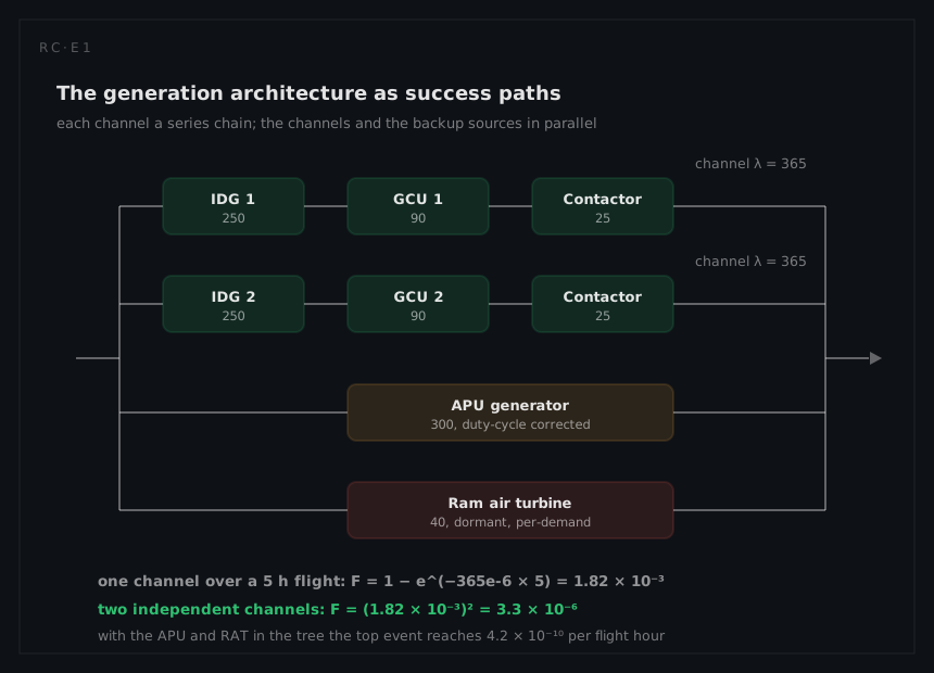
A single generation channel is a series chain: the generator, its control unit and the contactor that connects it to the bus. Series means every element must work, so the rates add:
λchannel = 250 + 90 + 25 = 365 per 10⁶ flight hours
Over a five-hour flight the channel's unreliability is
Fchannel(5) = 1 − e^(−365 × 10⁻⁶ × 5) = 1 − e^(−1.825 × 10⁻³) = 1.823 × 10⁻³
The exponential-of-a-sum shortcut hides what the series rule is doing, so it is worth writing out once. Each item survives the sector with probability e^(−λt), and the channel survives only if all three do:
RIDG(5) = e^(−250 × 10⁻⁶ × 5) = 0.998751 RGCU(5) = e^(−90 × 10⁻⁶ × 5) = 0.999550 Rcontactor(5) = e^(−25 × 10⁻⁶ × 5) = 0.999875
Rchannel(5) = 0.998751 × 0.999550 × 0.999875 = 0.998177
the same 1 − 1.823 × 10⁻³ by a longer road. Multiplying reliabilities and adding rates are one operation for exponential items and only for exponential items: the moment an element stops being exponential the product still works and the sum does not. Inverting the rate gives the mean the review will ask for:
MTTFchannel = 1 / (365 × 10⁻⁶) = 2,740 flight hours
which is 548 sectors between channel failures. The two channels roll up with their quantities visible:
| Item | λ each | Fitted in the success path | Contribution |
|---|---|---|---|
| Integrated drive generator | 250 | 2 | 500 |
| Generator control unit | 90 | 2 | 180 |
| Bus tie contactor | 25 | 2 | 50 |
| Generation chain, series total | 730 |
MTBFchain = 1 / (730 × 10⁻⁶) = 1,370 flight hours
At 3,000 flight hours a year that is 730 × 10⁻⁶ × 3,000 = 2.19 chain failures per aircraft-year, of which the generators contribute 2 × 250 × 10⁻⁶ × 3,000 = 1.5 removals. Those two figures, not the reliability, are what size the support system. The availability page takes the 1.5 into a sparing simulation; the maintainability page counts 755 per 10⁶ flight hours rather than 730, because the third contactor generates maintenance events without sitting in either success path.
Two channels of this kind sum without redundancy credit to 730 per 10⁶ flight hours, before the APU generator or the ram air turbine is given any credit at all. That number is the one people quote in reviews and it is almost meaningless on its own, because the aeroplane does not stop when a channel stops.
Step two: the architecture
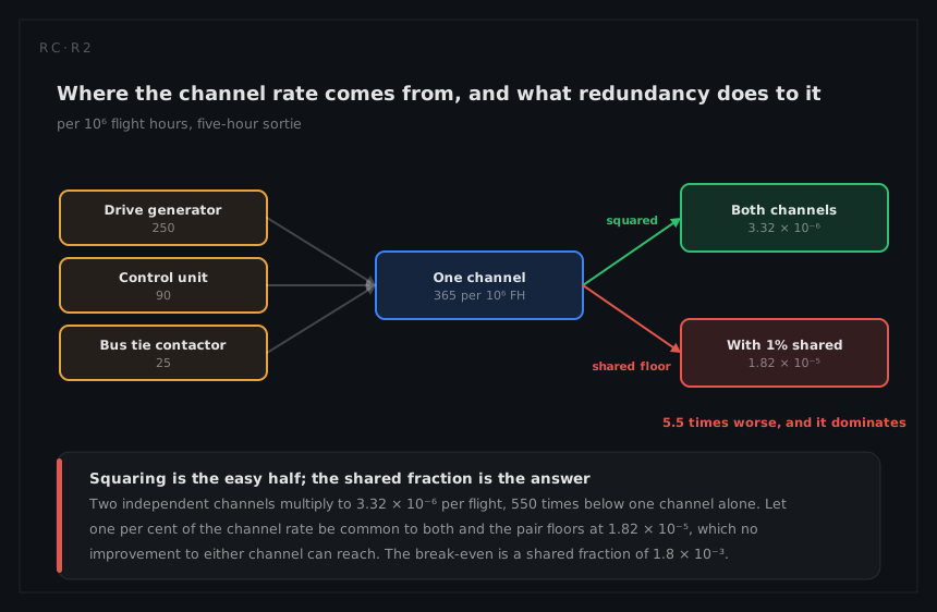
The two main channels are independent: different engines, different accessory gearboxes, separated routing, separate control units. Independent parallel means unreliabilities multiply:
Fboth channels(5) = (1.823 × 10⁻³)² = 3.32 × 10⁻⁶ per flight
At five hours a sector and 3,000 flight hours a year each aeroplane flies 600 sectors. Losing one channel or the other happens at
Feither channel(5) = 1 − (0.998177)² = 3.643 × 10⁻³
so 600 × 3.643 × 10⁻³ = 2.19 times a year, the same 2.19 the roll-up gave. Losing both arrives once in 1 / (3.32 × 10⁻⁶) = 301,000 sectors, or 502 aircraft-years. The same architecture produces an event twice a year and an event twice a millennium, and one multiplication separates them.
That is already a factor of 550 better than a single channel, from redundancy alone. Add the APU generator as a third source and the ram air turbine as a fourth, apply the mission profile properly (the APU's 300 per 10⁶ h is earned on the ground and in the fraction of flights where it runs, not across every flight hour, so it must be duty-cycle corrected before it is combined), and the assessed top event lands at 3.9 × 10⁻¹⁰ per flight hour, which is the figure the safety page derives and where the target it is measured against is set.
Both of those sources reach the tree already split into modes, and the split decides how much of each rate is genuinely an absent source. The APU's 300 resolves as 120 failure to start, 135 loss of output in the run and 45 degraded output; the turbine's 40 as 26 failure to deploy, 10 deploys with no output and 4 spurious deployment. Only the first two of each are losses of a power source.
Three readings the λ table does not contain
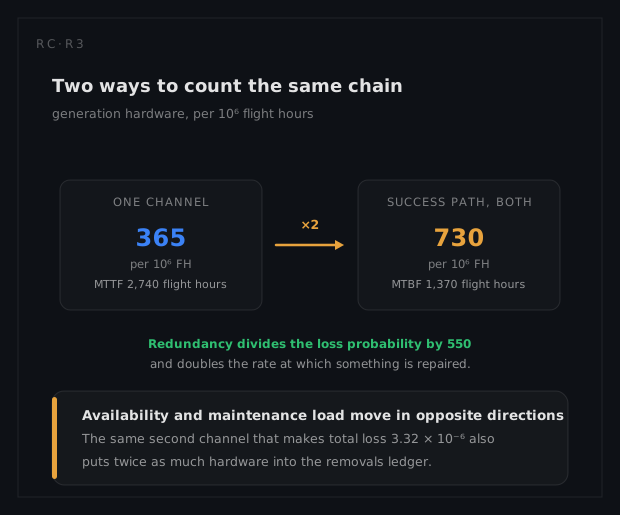
Three conclusions, in descending order of usefulness, and none of them is visible in the λ table.
The component rates barely matter. Halve the IDG rate from 250 to 125 and the channel drops to 240 per 10⁶ h, the channel unreliability to 1.20 × 10⁻³, and the two-channel figure to 1.44 × 10⁻⁶. A 50% improvement in the most expensive item in the system buys a factor of 2.3 in a number that redundancy already moved by 550. Money spent on component quality here is money spent on the wrong term.
Independence is the whole argument. The 3.32 × 10⁻⁶ assumes the two channels share nothing. They share a fuselage, a maintenance organisation, a fuel supply, and two identical part numbers. If even 1% of the channel failure rate is common to both, the pair's failure probability floors at 0.01 × 1.823 × 10⁻³ = 1.82 × 10⁻⁵, which is five and a half times worse than the independent calculation and now dominates it entirely. The break-even settles how much independence argument is enough: the two terms are equal at a shared fraction of 3.32 × 10⁻⁶ / 1.823 × 10⁻³ = 1.8 × 10⁻³, so any coupling above two parts in a thousand of the channel rate already dominates. This is why the analysis that decides this design is not the RBD but the common cause work described on the safety page.
The dormant source is not what it seems. The ram air turbine contributes 40 per 10⁶ h, the second-smallest number in the table, and it is the item most likely to invalidate the whole argument, because nobody would know it had failed. Its reliability question is not its rate but its detectability, which the testability page takes up with the proof-test arithmetic.
What the analysis tells the engineer to do
Four decisions follow, and every one of them is priced by a number computed above.
Spend the reliability budget on separation, not on parts. Halving the generator's rate is a multi-year component programme and buys a factor of 2.3. Holding the common-cause fraction below the 1.8 × 10⁻³ break-even is what buys the factor of 550, and it is bought with separate gearboxes, separated routing, independent buses and dissimilar control-unit software. Only the second purchase can be lost by an oversight rather than by a deliberate choice.
Treat the turbine's check interval as a design parameter. Its dormant unavailability is set by the interval, not by the item:
QRAT = λT / 2 = 36 × 10⁻⁶ × 500 / 2 = 9.0 × 10⁻³
The rate is the turbine's 36 per 10⁶ hours of silent modes rather than its whole 40, because the spurious-deploy mode is caught by continuous built-in test and never lies latent between checks. Halving the interval to 250 flight hours halves the term to 4.5 × 10⁻³. Halving the turbine's own silent rate from 36 to 18 per 10⁶ hours buys the identical factor of two and costs a hardware programme, while the interval costs a line in the maintenance schedule.
Ship the removal rate downstream, not the reliability figure. The 2.19 chain events and 1.5 generator removals per aircraft-year size the spares pool, the technician load and the dispatch argument, and no reader can reconstruct them from an MTBF without the 3,000-hour utilisation beside it.
Keep the hard time on the drive, and set it from the crossover. The drive mechanical mode carries 15% of the generator's rate on the safety worksheet, so 0.15 × 250 = 37.5 per 10⁶ flight hours, 10.3% of the channel's 365: small enough to ignore while the drives are young, large enough to matter when they are not. The section below finds the age at which the two candidate models change places, and a removal interval set below it is what keeps every exponential on this page conservative.
What a different technique would have given
Had the drive been modelled with the Weibull it deserves rather than the exponential it was given, the late-life picture would change materially. A drive with β around 2 and a characteristic life near the airframe's overhaul interval has a hazard that is well below the constant assumption early and well above it late; the constant-rate model spreads that unevenness into a flat average that is wrong at both ends and right only in the middle.
The shape of that disagreement deserves numbers. The drive mode's 37.5 per 10⁶ flight hours implies a mean life of 1 / (37.5 × 10⁻⁶) = 26,667 hours. Hold that mean fixed and give it β = 2:
MTTF = η · Γ(1 + 1/β) = η · Γ(1.5) = 0.8862 η η = 26,667 / 0.8862 = 30,100 flight hours
Nothing here is fitted and nothing can be, because no fleet has flown; this is one mean life carried by two shapes, which is all the choice of model ever amounts to. The tenth percentiles part company at once:
B10 (Weibull) = η(−ln 0.9)^(1/β) = 30,100 × (0.10536)^(1/2) = 9,770 flight hours B10 (exponential) = −ln(0.9) / λ = 0.10536 / (37.5 × 10⁻⁶) = 2,810 flight hours
The two hazards agree at exactly one age, from (β/η)(t/η)^(β−1) = λ:
t* = λη² / 2 = 37.5 × 10⁻⁶ × 30,100² / 2 = 17,000 flight hours
a little under six years at 3,000 flight hours a year. Below it the constant rate is pessimistic: at 5,000 hours the Weibull hazard is (2 / 30,100)(5,000 / 30,100) = 11.0 per 10⁶ against the 37.5 assumed. Above it the constant rate is optimistic: at 30,000 hours it is 66.2 per 10⁶, 1.77 times the assumption. Carry that into the channel, 365 − 37.5 + 66.2 = 393.7 per 10⁶, giving 1 − e^(−393.7 × 10⁻⁶ × 5) = 1.967 × 10⁻³ and
Fboth channels(5) = (1.967 × 10⁻³)² = 3.87 × 10⁻⁶
against the 3.32 × 10⁻⁶ the report carries. Sixteen per cent worse, on an aeroplane whose analysis says nothing has changed.
The programme handles this not by improving the model but by removing the problem: the hard-time limit retires the drive before the rising hazard arrives, which converts a wear-out item into an effectively constant-rate one over the interval that matters. That is a legitimate and common engineering answer, and it is worth recognising it for what it is, a maintenance policy substituting for a distribution. It works because a retirement age below 17,000 flight hours is affordable here; where no such age exists, the distribution has to be modelled rather than legislated away.