

Six hundred volumetric infusion pumps in one hospital, each running about 2,500 hours a year. A pumping mechanism, an occlusion sensor, an air-in-line detector, a dose controller and a rechargeable battery. The fleet generates enough returns to fit distributions properly, and the first fit produced is wrong in an instructive way, which is what this page is about.
The technique, and why this one
Field-data fitting with the population separated by mechanism before any distribution is fitted. The hospital's biomedical department has years of work orders, so prediction is unnecessary. What is necessary is resisting the temptation to fit the fleet as a whole.
| Item | Model | Parameters | Note |
|---|---|---|---|
| Pumping mechanism | Weibull | β = 1.6, η = 3,700 operating h | plunger-drive wear |
| Battery | Weibull | β = 3.4, η = 5,300 calendar h | strong wear-out, on a replacement cycle |
| Occlusion sensor | exponential | λ = 150 per 10⁶ h | no wear signature |
| Air-in-line detector | exponential | λ = 120 per 10⁶ h | no wear signature |
| Dose controller board | exponential | λ = 90 per 10⁶ h | electronics in useful life |
Three items keep a constant rate and two do not, and the split is not a matter of taste. The sensors and the controller board are screened electronics in a temperature-controlled building well inside their useful life, the one condition under which the exponential model is a description rather than a convenience; the storage array controller page makes that choice for a whole system and defends it. The drive and the battery fail by accumulating damage, so their hazard is a function of age and an exponential fit discards the only variable a policy can act on. The Weibull items carry 1,100 of this pump's 1,460 per 10⁶ hours: three quarters of the failure rate sits on items whose hazard is moving, the reverse of the storage array, which is why the two pages end up opposite.
The mixed-population trap
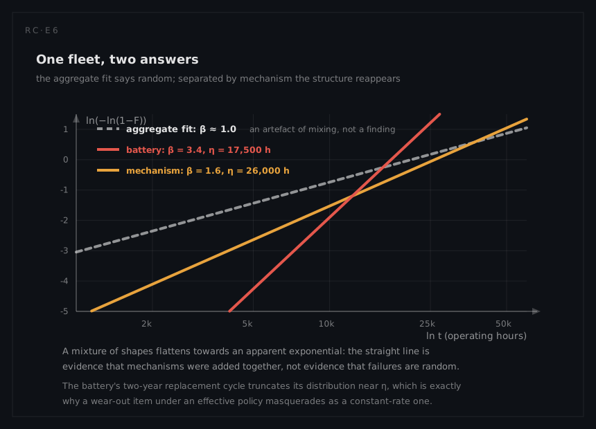
Take every pump return from the fleet, rank them, and fit a single Weibull. The result comes out close to β = 1.0, and it looks clean: a straight line on the probability plot, a comfortable interpretation that pump failures arrive at random, and a clear conclusion that preventive maintenance beyond the statutory annual service would be wasted money.
That conclusion is an artefact. A mixture of several distributions with different shapes and different characteristic lives tends to flatten towards an apparently exponential aggregate, because the early failures of the steep population overlap the later failures of the shallow one and the combination washes out both curvatures. The straight line is not evidence of randomness; it is evidence that several mechanisms have been added together.
Separate the returns by the part that actually failed and the structure reappears:
- The battery fits β = 3.4, η = 5,300 calendar hours. That is aggressive ageing: charge cycling degrades capacity, and the hazard climbs as the square and a bit of age.
- The pumping mechanism fits β = 1.6, η = 3,700 operating hours. A mild wear-out on the plunger drive, real but far less urgent.
- The sensors and the controller board show no curvature at all and keep their constant rates honestly.
Where the two curves put their failures
A shape is only worth fitting once percentiles are read off it, because a percentile is what a replacement interval is written in:
tp = η(−ln(1 − p))^(1/β)
For the plunger drive at β = 1.6, η = 3,700 operating hours:
B10 = 3,700 × (0.10536)^(1/1.6) = 3,700 × 0.2450 = 907 h
B50 = 3,700 × (0.69315)^(1/1.6) = 3,700 × 0.7953 = 2,943 h
MTTF = η·Γ(1 + 1/β) = 3,700 × Γ(1.625) = 3,700 × 0.8966 = 3,317 h
At 2,500 hours a year: four and a half months to the first tenth of the population, fourteen to the median, sixteen to the mean, and the average rate that follows, 10⁶/3,317 = 301 per 10⁶ operating hours, is the 300 the fleet ledger carries. The battery at β = 3.4 is far tighter, with B10 = 5,300 × 0.51588 = 2,734 hours and a mean of 5,300 × Γ(1.2941) = 4,761 hours falling within three hours of its own median, both of them short of the 5,300-hour replacement date. A high β is a narrow distribution, which is what makes a scheduled replacement worth setting at all.
The hazard rate says it in the planner's units:
h(t) = (β/η)(t/η)^(β−1) so h(2t)/h(t) = 2^(β−1)
plunger drive 2^0.6 = 1.52 battery 2^2.4 = 5.28 any exponential item 2^0 = 1
The testability page evaluates the battery ratio directly, 122 per 10⁶ hours at half the cycle rising to 642 at the replacement point. The third line decides more policy than the other two: for the electronics the ratio is one at every age, so no life limit could reach them.
Why the battery hides so well
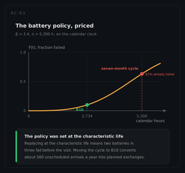
The battery's characteristic life is 5,300 hours. The hospital replaces batteries on a seven-month cycle, which at 2,500 operating hours a year is only 1,513 hours, far out on the shallow left tail where barely one battery in seventy has failed; expressed against calendar time on a 24-hour-a-day ward pump the same cycle is 5,300 hours, essentially η itself. Either way, the policy truncates the distribution before most of its mass arrives, so the observed battery failures are the left tail of a steep curve, and a left tail of a steep Weibull looks very much like a flat rate.
The battery ages on the wall clock whether the pump runs or not, so the replacement date is 5,300 calendar hours, which is η itself:
F(5,300 calendar h) = 1 − exp(−(5,300 / 5,300)^3.4) = 1 − exp(−1) = 0.632
A pump reaches its replacement date with nearly two thirds of its batteries already gone, the figure the safety page works from. Reading the same interval against the 1,513 operating hours the pump accumulates in those seven months would return 0.014, forty-five times smaller and simply the wrong clock for an item that ages on the shelf.
This is the general trap worth carrying away: a wear-out item under an effective replacement policy masquerades as a constant-rate item in the aggregate data. The policy is doing the work, the data has been shaped by the policy, and an analyst who removes the policy on the strength of the data will rediscover the distribution the hard way.
Rolling the fleet up
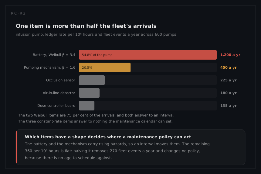
For the fleet arithmetic the two Weibull items enter at the book rates the maintenance ledger carries for them, 300 per 10⁶ hours for the mechanism and 800 for the battery, with the constant items as listed, giving 1,460 per 10⁶ hours per pump. Both are the average rates of the fitted distributions above, converted to the pump's operating clock: the mechanism's 10⁶/3,317 = 301, and the battery's two handling events a pump-year, which on 2,500 operating hours is 800. The ledger counts maintenance actions rather than failures alone, so the battery's 1,200 divides into the 758 that arrive as failures before the scheduled date and the 442 exchanged on policy; both occupy the bench, which is why the workshop is sized on the sum. At 2,500 operating hours that is 3.65 events per pump-year, and across 600 pumps roughly 2,190 events a year arriving at one biomedical department.
| Item | λ per 10⁶ h | Share of pump rate | Fleet events a year |
|---|---|---|---|
| Battery | 800 | 54.8% | 1,200 |
| Pumping mechanism | 300 | 20.5% | 450 |
| Occlusion sensor | 150 | 10.3% | 225 |
| Air-in-line detector | 120 | 8.2% | 180 |
| Dose controller board | 90 | 6.2% | 135 |
| Pump total | 1,460 | 100% | 2,190 |
The last column is the rate column times 1.5, since 600 pumps at 2,500 hours is 1.5 × 10⁶ pump-hours a year. The three constant-rate rows are the only ones that behave as a textbook series calculation assumes, and over an operating year they multiply out term by term:
RE(2,500) = e^(−150×10⁻⁶×2,500) × e^(−120×10⁻⁶×2,500) × e^(−90×10⁻⁶×2,500) = 0.687 × 0.741 × 0.799 = 0.407
so 0.9 electronic failures per pump-year, 540 across the fleet, and a 59% chance a given pump sees one. That block will not worsen with age and answers to no interval.
The aggregate is also measured very precisely, which is the last part of the trap. With 2,190 events a year the count is Poisson, so a 90% interval is 2,190 ± 1.645√2,190 = 2,190 ± 77 and the pump rate is pinned to
1,460 × (1 ± 0.035) = 1,409 to 1,511 per 10⁶ h
three and a half per cent either side, and it was that well determined before anyone separated the population. The aggregate fit was precise and wrong at the same time, and no confidence interval warns you, because the interval is computed on the quantity you chose to estimate and never on the choosing.
At nearly nine events a working day the department behaves like a queue rather than a workshop, and the operational consequence of a reliability improvement becomes nonlinear: shaving 20% off the arrival rate shortens the backlog by considerably more than 20%, because the department was operating near its service capacity. That is the point at which a reliability number stops being a property of the device and becomes an input to an operations model, and the availability page picks it up there, with and without the loaner pool. The maintainability page enlarges the same 2,190, because 17% of what reaches the bench has nothing wrong with it: 2,190 / 0.83 = 2,640 units arrive a year, about 450 of them healthy and consuming a full service time regardless.
What the number does not cover
The dominant hazard of this device is over-infusion, and the analysis on the safety page finds that device failures cause a minority of it: most over-infusion events begin with a correctly functioning pump programmed wrongly. A reliability improvement programme aimed at the 1,460 per 10⁶ hours would leave roughly four fifths of the harm untouched.
That is not a criticism of the reliability work; it is a statement about scope. The 1,460 is the right answer to the question "how often does this device fail", and the device's most important risk is not answered by that question. Recognising which of your numbers is authoritative for which decision is most of the skill.
What the analysis tells the engineer to do
Change the battery at B10 rather than at η. The comparison is 0.632 of the population failed at the scheduled 5,300 hours against 0.10 at 2,734, on an item worth 1,200 of the 2,190 fleet events a year, 758 of them unscheduled. The battery itself does not improve; what changes is which side of the schedule its work lands on, and the availability page turns that into utilisation and ward-visible downtime.
Forecast the plunger drive against fleet age instead of holding it flat. B10 at 907 operating hours is four and a half months and the hazard rises 1.52 times per doubling of age. Replacing at B10 is not the answer, since that exchange is a workshop job; the flat arrival forecast is the thing that is wrong, and a fleet bought in one procurement will deliver its mechanism failures as a wave.
Spend nothing on the electronics. Those three items are 360 per 10⁶ hours, 24.7% of the pump, at a hazard ratio of one at every age. Halving all three removes 270 fleet events from 2,190 and changes no policy, because there is no interval to set against a flat hazard. Their leverage is detection, which the testability page works.
Require the work order to name the part. Every decision above rests on one field distinguishing five items; without it the only fit is the fleet fit, the only answer β ≈ 1.0, and the finding that nothing needs a schedule.
What a different technique would have given
Accepting the aggregate β ≈ 1.0 would have produced three wrong decisions in sequence: that preventive battery replacement is unnecessary (it is the single most effective maintenance action on this fleet), that the plunger drive needs no life limit (it has a real, if mild, ageing mechanism), and that the failure arrival rate will stay flat as the fleet ages (it will not, because two of the five contributors are climbing). The fit was not incorrect arithmetic. It was correct arithmetic on the wrong population, which is harder to catch and does more damage.