

Two brake ECUs, an electro-hydraulic actuator, four wheel-speed sensors and an independent backup hydraulic path, multiplied by two hundred thousand vehicles. This is the one system in the set large enough that reliability stops being predicted and starts being measured, and the page is about that handover: what changes when the warranty database can answer the question better than the handbook can.
The technique, and why this one
Maximum-likelihood Weibull fitting to warranty returns, with the surviving fleet carried as suspensions, and B10 rather than a mean as the requirement currency. At design time the actuator carried a predicted 180 per 10⁶ hours from a parts-count model. Twenty-four months into production there are enough returns to fit a distribution, and the fit answers a question the point prediction never could: not how often, but when and in what pattern.
| Item | Model at design | Model in service | Why it changed |
|---|---|---|---|
| Electro-hydraulic actuator | exponential, λ = 180 per 10⁶ h | Weibull, β = 1.4, η = 9,500 h | returns show a rising hazard |
| Brake ECU | exponential, λ = 60 per 10⁶ h | exponential, unchanged | no wear signature in the returns |
| Wheel-speed sensor set | exponential, λ = 90 per 10⁶ h | exponential, unchanged | no wear signature |
| Backup hydraulic path | exponential, λ = 20 per 10⁶ h, dormant | unchanged | too few demands to fit |
Summed in series, 60 × 2 + 180 + 90 + 20 = 410 per 10⁶ hours, the last figure here a handbook can supply and the one the rest of the row starts from: 0.195 vehicle-off-road incidents a vehicle-year on the availability page, 41,000 corrective events a year on the maintainability page, a 390-plus-20 split into primary and backup legs on the safety page.
The electronic rows keep their constant rates for the reasons the storage array page defends the exponential across an entire system: screened parts, a controlled environment, a service life shorter than the onset of anything in them that wears. The actuator is a pump, a valve block and a set of seals that stroke every time the driver brakes, and it meets none of those conditions. A parts-count model cannot see the difference, because MIL-HDBK-217F, IEC TR 62380 and SN 29500 alike address the flat middle of the bathtub curve and nothing else. Asking a constant-rate prediction whether an item wears out is asking a question the model was built unable to answer.
Censoring is the whole problem
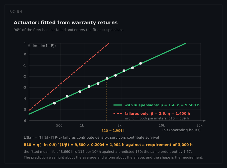
At 500 operating hours a year, a fleet two years into production has accumulated roughly 1,000 hours per vehicle, and the overwhelming majority of vehicles have not failed. Any fit that uses only the failure times is answering the question "given that a unit failed, when did it fail", which is not the question anyone asked. The surviving units are right-censored observations and they carry most of the information in the sample.
The likelihood carries both populations: each failure contributes its density f(tᵢ), each survivor contributes its survival R(tⱼ), and the parameters are those that maximise the product
L(β, η) = Π f(tᵢ) · Π R(tⱼ)
Maximising over the actuator returns gives β = 1.4, η = 9,500 hours. Fitting the failures alone, as an analyst in a hurry might, returns something close to β = 2.6 with η near 1,400 hours: a far more alarming shape and a far shorter life, both artefacts of throwing away the survivors.
What the fit says that the prediction could not
The design-stage constant of 180 per 10⁶ hours was not badly wrong about the average. The fitted mean life is
MTTF = η · Γ(1 + 1/β) = 9,500 × Γ(1.714) = 9,500 × 0.9114 = 8,660 h
which is 115 per 10⁶ hours, the same order as the prediction. The prediction was wrong about the shape, not the average, and the shape is what the requirement is written against.
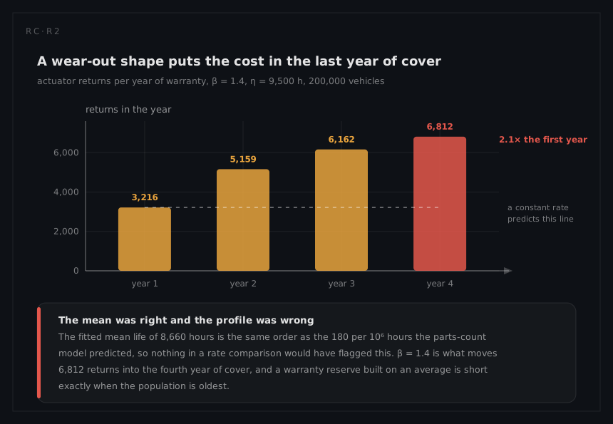
β = 1.4 is a mild but unmistakable wear-out. Failures are not arriving uniformly across the fleet's age; they are concentrating in the older vehicles, which means the warranty exposure grows faster than a linear projection and the third and fourth years of cover cost disproportionately more than the first two.
That is a quantity, not a remark. Take F(t) = 1 − e^(−(t/9,500)^1.4) at the end of each year of cover, across 200,000 vehicles:
| Year | Hours | F(t) | Failed to date | Failed in the year |
|---|---|---|---|---|
| 1 | 500 | 1.61% | 3,216 | 3,216 |
| 2 | 1,000 | 4.19% | 8,375 | 5,159 |
| 3 | 1,500 | 7.27% | 14,537 | 6,162 |
| 4 | 2,000 | 10.67% | 21,349 | 6,812 |
A constant rate puts the same number in every cell. This one puts 2.1 times as many actuators in the fourth year as in the first.
The requirement is a B10 life, and that is where the design fails:
B10 = η · (−ln 0.9)^(1/β) = 9,500 × (0.10536)^(1/1.4) = 9,500 × 0.2004 = 1,904 h
about four years of typical driving, against a requirement of B10 ≥ 3,000 hours. The design meets its average and misses its percentile, which is exactly the failure mode a mean-based requirement is blind to and the reason this industry writes B-lives instead. The reliability foundations make the general argument; this is what it costs in practice.
Other percentiles come from the same expression, tp = η · (−ln(1 − p))^(1/β), and the first-year one is the sharpest: B1 = 9,500 × (0.01005)^(1/1.4) = 9,500 × 0.0374 = 355 hours, so one vehicle in a hundred loses its actuator inside its first year of cover. The fit itself is not in doubt at this sample size: 4.19% failed by 1,000 hours is a binomial proportion on 200,000 vehicles, standard error √(0.0419 × 0.9581 / 200,000) = 4.5 × 10⁻⁴, which holds η to ±0.78% and B10 between 1,889 and 1,919 hours. The shortfall against 3,000 is more than thirty times the sampling error.
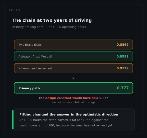
A fit on one item becomes an answer only once it is composed with the chain around it, and at two years of driving the primary path multiplies terms from both distributions:
RECUs = e^(−120 × 10⁻⁶ × 1,000) = 0.8869
Ractuator = e^(−(1,000/9,500)^1.4) = e^(−0.0428) = 0.9581
Rsensors = e^(−90 × 10⁻⁶ × 1,000) = 0.9139
Rprimary(1,000 h) = 0.8869 × 0.9581 × 0.9139 = 0.777
The actuator term audits the fit: 4.2% failed by 1,000 hours is the 96% not-failed the sample showed. Put the design constant back and that term becomes e^(−0.180) = 0.8353, the chain 0.677, ten points pessimistic about a fleet whose fitted hazard at that age is only 60 per 10⁶ hours.
Fleet scale changes the economics of everything
At 200,000 vehicles and 500 hours a year, the series sum of 410 per 10⁶ hours is 0.205 failures per vehicle-year before any redundancy credit, which is 41,000 warranty events a year from a rate that would be unremarkable on a single machine. Two consequences follow that no single-unit analysis surfaces.
Improvement pays back at fleet scale, so the threshold for acting is far lower. A change that shifts the actuator's η from 9,500 to 13,000 hours moves B10 from 1,904 to 2,605 hours and cuts four-year warranty incidence by roughly a third: F(2,000) = 1 − e^(−(2,000/13,000)^1.4) = 7.02% against 10.67%, or 14,036 returns in the first four years instead of 21,349. On one vehicle that is a rounding error; across the fleet those 7,313 units are a line item large enough to fund the redesign several times over.
The data arrives fast enough to be actionable, so the prediction's job is to be temporary. The programmes that handle this well plan the handover deliberately: predict to set the targets, measure to correct them, and stop quoting the prediction once the field has spoken. The programmes that handle it badly leave the design-stage 180 per 10⁶ hours in the reliability report for the life of the model, long after the returns have contradicted its shape.
The dormant path, and what this analysis cannot see
The backup hydraulic path contributes 20 per 10⁶ hours, the smallest number in the table, and the fit cannot say anything useful about it, because it is exercised only when the primary fails and there are almost no demands in the record. Its reliability question is not its rate but whether a failed backup would be noticed before it was needed, which is a detection question rather than a distribution question and belongs to the testability page. The severity of getting it wrong belongs to the safety page, where the same hazard is assessed for severity, exposure and controllability and lands on the highest automotive integrity level.
What the analysis tells the engineer to do
Size the actuator fix against the percentile. B10 is linear in η, so B10 ≥ 3,000 hours needs η = 3,000 / 0.2004 = 14,970 hours, a 58% increase. The 13,000-hour candidate removes 7,313 returns and still lands 395 hours short, and knowing that before the change is authorised is the difference between a fix and a partial one sold as a fix.
Budget the warranty on the profile, not on a rate. The fourth year of cover carries 6,812 actuator events against the first year's 3,216, so a reserve built on 0.205 incidents per vehicle-year is under-funded exactly when the model is oldest. The same young-fleet figure is spent downstream by every other page in this row, and none of them re-runs unless somebody schedules it.
Hand the shape to a monitor. With β = 1.4 degradation precedes failure, and the hazard climbs from 45 to 79 per 10⁶ hours between the first and fourth years of driving, so a trend on the actuator's pressure-rise time has something to watch that a threshold has not.
What a different technique would have given
Keeping the exponential and reporting 115 per 10⁶ hours from the field data would have produced a defensible-looking average, a B10 of −ln(0.9)/λ = 916 hours (worse than the Weibull says, because the exponential front-loads failures the actuator does not actually have), and no signal at all that the hazard is rising. At the percentile the first year is judged on it is worse still: B1 = 0.01005 / 115 × 10⁻⁶ = 87 h against the fitted 355. The programme would have concluded that its actuator is roughly as predicted, that preventive replacement is pointless, and that warranty exposure scales linearly with time in service. All three conclusions are wrong, and the third is the one that shows up in the accounts.