

Four reaction wheels of which three are needed, two star trackers, three magnetorquers and an onboard computer with a cold spare. Seven years in orbit, no repair, and every reliability decision made before the launch vehicle leaves the pad. This is the purest survival problem in the set: there is no MTBF-against-MTTR trade to make, only the area under the curve.
The technique, and why this one
Monte Carlo simulation, because the closed form runs out before the question does. The wheels wear, so they are Weibull rather than exponential, and a k-out-of-n arrangement of identical Weibull items is still analytically tractable. What is not tractable is what the operations concept adds on top: when a wheel fails, the ground reassigns control across the remaining three in a degraded pointing mode, and that reconfiguration takes 7.2 hours and can itself fail. Once the system's behaviour depends on a sequence of events with their own distributions and their own failure probabilities, the structure stops being a static block diagram and simulation becomes the honest tool.
The discipline here is worth stating plainly: do not simulate what you can integrate. The closed form is computed first, both because it is exact and because it is the check that the simulation is not lying.
| Item | Model | Parameters | Redundancy |
|---|---|---|---|
| Reaction wheel | Weibull | β = 2.2, η = 15 years (131,400 h) | 4 fitted, 3 required |
| Star tracker | exponential | λ = 4 per 10⁶ h | 2 fitted, 1 required |
| Magnetorquer | exponential | λ = 1 per 10⁶ h | 3 fitted, 2 required |
| Onboard computer | exponential | λ = 2 per 10⁶ h | 1 + cold spare at 10% λ |
Those rates are two orders of magnitude below the terrestrial figures elsewhere in this chapter. That is not optimism; it is what screened, derated, single-lot parts in a benign thermal-vacuum environment cost, and the programme paid for every decimal place.
They are also deliberately not the 150, 60 and 200 per 10⁶ hours that the safety and testability pages carry for the same three items. Those are design-stage constants chosen to weight coverage and consequence sums, where what matters is the ratio between items rather than the absolute level. These are flight-lot life rates, and mission survival is the one calculation that needs the absolute level to be right. A number is only meaningful with its purpose attached, and the same item legitimately carries different rates in a coverage roll-up and in a survival integral.
Step one: the closed form
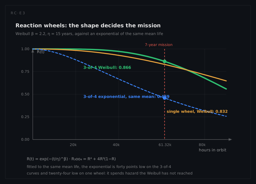
A single wheel's reliability at the seven-year point (61,320 hours) is
R(t) = exp(−(t/η)^β) = exp(−(61,320 / 131,400)^2.2) = exp(−(0.4667)^2.2) = exp(−0.1870) = 0.829
Two parameters fix the whole life. Using tp = η·(−ln(1 − p))^(1/β),
B10 = 131,400 × (0.10536)^(1/2.2) = 131,400 × 0.3595 = 47,240 h (5.4 years)
The mission therefore ends past B10 and short of the 111,200-hour median, η × (ln 2)^(1/2.2): the population is visibly failing but mostly alive, which is the only region where a k-out-of-n spare earns anything.
Because all four wheels are the same design, the same age and the same distribution, the three-out-of-four arrangement has an exact binomial form:
R3oo4 = R⁴ + 4·R³·(1 − R)
R3oo4 = 0.4733 + 4 × 0.5707 × 0.1705 = 0.4733 + 0.3893 = 0.863
The remaining terms are the mission-losing ones: 6R²(1 − R)² = 0.1201, 4R(1 − R)³ = 0.0165, (1 − R)⁴ = 0.0008, totalling 0.1374, the branch the safety page treats as dominant. Expected failures are 4 × (1 − 0.829) = 0.68, and 1 − 0.4733 = 0.527 of missions use the spare.
The other three blocks are exponential, each with its own structural form:
RST = 1 − (1 − e^(−4×10⁻⁶ × 61,320))² = 1 − (1 − 0.7825)² = 1 − 0.0473 = 0.9527
RMT = R³ + 3R²(1 − R), R = e^(−1×10⁻⁶ × 61,320) = 0.9405, so 0.8319 + 0.1579 = 0.9898
ROBC = e^(−λt)(1 + λt) = 0.8846 × 1.1226 = 0.9931
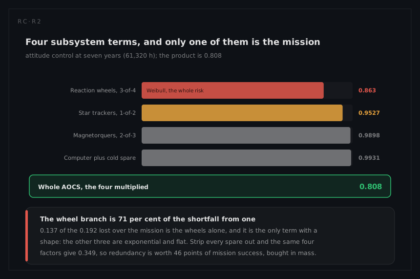
The star trackers, magnetorquers and computer contribute 0.9527, 0.9898 and 0.9931 respectively, so the subsystem reliability is
RAOCS = 0.863 × 0.9527 × 0.9898 × 0.9931 = 0.808
The same four factors with every spare stripped out give 0.5707 × 0.7825 × 0.8846 × 0.8846 = 0.349, so redundancy is 46 points of mission success on this vehicle, bought entirely in mass.
Why the wheels are Weibull and the rest are not
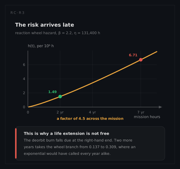
Two models sit in the same table and the split is not a matter of taste. A constant hazard is correct when service life is deliberately shorter than the onset of any wear mechanism the item owns, the defence made at length for the controller boards in the electronics page. The trackers, magnetorquers and processor pass that test: solid state, thermal vacuum, nothing inside them rubbing on anything else. The wheels fail it, because they have bearings, the bearings have lubricant, and the lubricant degrades on a clock indifferent to when the mission ends:
h(t) = (β/η)(t/η)^(β−1) = 1.674 × 10⁻⁵ × (t/131,400)^1.2
h(17,520) = 1.674 × 10⁻⁵ × 0.0891 = 1.49 × 10⁻⁶ per hour
h(61,320) = 1.674 × 10⁻⁵ × 0.4007 = 6.71 × 10⁻⁶ per hour, a factor of 4.5 higher
One distribution for both populations would have been wrong in opposite directions. An exponential flattens the wheel hazard exactly where the mission needs it; a Weibull on the electronics would manufacture a wear-out signature the parts do not have. That ramp is an asset in the testability column, where a hazard with years to run is a trend telemetry can watch.
Step two: what simulation adds
The closed form assumes that losing a wheel is instantaneous in its effect and that three wheels are simply three wheels. Neither is quite true. The real sequence is: a wheel degrades, telemetry reveals it, the ground diagnoses and decides, a reconfiguration is uplinked, and the spacecraft resumes in a degraded mode with reduced slew authority. Each step has a duration and a probability of not completing.
A Monte Carlo model samples, for each of 100,000 synthetic missions, a failure time for every wheel from the Weibull, exponential times for the other items, a reconfiguration duration and a reconfiguration success draw, then plays the mission forward and records whether the imaging service survived seven years. The result is a mission success probability of 0.81, with a 95% confidence interval of 0.808 to 0.812 on 100,000 runs, agreeing with the closed form to three digits while additionally producing what the closed form cannot: the distribution of the number of wheel failures per mission, the distribution of time spent in degraded pointing, and the sensitivity of the answer to reconfiguration reliability.
The convergence is worth noting, because it is the practical constraint on this technique. The standard error of a simulated probability p over n runs is √(p(1−p)/n), which at the run count used is
SE = √(0.81 × 0.19 / 100,000) = 1.24 × 10⁻³, half-width 1.96 × SE = 2.4 × 10⁻³
the interval quoted above and nothing tighter. At p ≈ 0.81 reaching a standard error of 0.001 needs about 154,000 runs, and reaching 0.0001 needs 15.4 million. Simulation buys generality at a fixed price in precision per run, which is why it is the wrong tool for the 10⁻⁹ questions in the aerospace page and the right one here.
The design decision the shape drives
With β = 2.2 the hazard rises steeply through the mission, and that changes where the fourth wheel earns its keep. In the first two years the wheels are almost certain to survive and the spare contributes almost nothing; in the last two years the per-wheel hazard has climbed enough that the spare is carrying the mission. The arithmetic is blunt:
F(0 → 17,520 h) = 1 − exp(−(0.1333)^2.2) = 1 − 0.9882 = 0.0118
F(43,800 → 61,320 h) = R(43,800) − R(61,320) = 0.9147 − 0.8295 = 0.0852
Seven times the risk in the same two years of calendar. The correct reading is that the redundancy is a late-life asset, which in turn means the mission extension conversation, always tempting when a spacecraft is healthy at end of design life, is precisely the conversation in which the spare is already spent.
The cold spare computer illustrates the opposite trap. Held unpowered at a tenth of its active rate it accumulates almost no risk while waiting, and the arithmetic rewards it handsomely. Carrying the dormant rate explicitly, R = e^(−λt)[1 + (λ/λd)(1 − e^(−λd·t))], costs that block 0.9931 − 0.9924 = 0.0007, inside the simulation's own interval. What the arithmetic does not contain is whether the changeover works: a spare that has not been exercised in six years, switched by a bus that must itself be healthy, is a mechanism whose failure mode is not covered by its dormant rate. Flight software exercises the redundancy on a schedule for exactly this reason, and the testability page treats telemetry as the only test access this system will ever have.
What the analysis tells the engineer to do
Carry the fourth wheel, and justify it on the last two years. Three wheels with no spare give 0.8295³ = 0.571 at seven years and the fourth takes the branch to 0.863, so the spare is worth 0.292 of mission success. Nothing else here moves the answer that far, and almost all of it is earned after year five.
Gate any mission extension on wheel age, not on payload health. The mission ends at the B17 point of the population (1 − 0.829 = 0.171), already past the 47,240-hour B10. The safety column runs the same Weibull two years further to 0.691, a B28 population, taking the wheel branch from 0.137 to 0.309. The gate is a re-run of this calculation, and it costs nothing to write into the operations plan before launch.
Spend the next analysis hour on reconfiguration success, not on more runs. Driving the standard error from 1.24 × 10⁻³ to 10⁻⁴ costs 15.4 million runs and buys decimal places on an answer whose leading uncertainty is a human procedure with no second attempt. The maintainability column takes those 7.2 hours apart into three lognormal stages summing to 7.35.
Hand the 0.81 on as a multiplier. The availability column multiplies it by the 0.983 imaging-service figure to get 0.796, which is what a customer receives across the mission, and the safety column reads its complement, 0.19, as the probability that the vehicle cannot control its attitude when the deorbit burn falls due.
What a different technique would have given
Fitting an exponential with the same mean life as the Weibull (η·Γ(1 + 1/β) = 131,400 × Γ(1.4545) = 131,400 × 0.8856 = 116,400 h, so λ = 8.6 per 10⁶ h) gives a per-wheel reliability at seven years of e^(−0.527) = 0.590 and a 3-out-of-4 value of 0.459. Fitting one to the same seven-year point instead reproduces 0.829 per wheel and 0.863 for the array at that one instant by construction, and is wrong at every other age. Neither exponential reproduces both ends, and that is the general result: an exponential fitted to a wear-out population can be made correct at one point in time and is wrong everywhere else. For a mission whose whole question is what happens at a specific age, that is not a small error.