

Four reaction wheels of which three are required, two star trackers, three magnetorquers and an onboard computer with a cold spare, in a seven-year orbit that no engineer will ever visit. Every other system in this chapter can be opened, probed, removed or replaced if the built-in test proves inadequate. This one cannot. Whatever observability is designed into it before launch is the entire diagnostic capability it will have for the rest of its existence.
That turns the usual testability question inside out. Elsewhere the question is how much of the failure population the test means catch, with the unspoken assumption that the residue will eventually be found some other way. Here there is no other way. A failure mode that produces no telemetry signature is not merely undetected; it is permanently undiagnosable, and the recovery procedure that would have depended on knowing about it does not exist. Coverage is therefore not a maintenance economy on this spacecraft, it is a survival property, and it competes for resources with the payload.
The technique, and why this one
A dependency matrix in which the cost column is bits per second: observability designed against the downlink budget, with each candidate monitor scored by the failure rate it moves from undetected to detected per unit of bandwidth consumed. The technique is chosen because the binding constraint is not sensor cost or processing margin, which are the usual limits, but the housekeeping share of the downlink, fixed at 4% of the total. Every parameter telemetered is payload data not returned, for seven years, and the trade is permanent in a way that no ground-testable system ever faces.
| Item | λ per 10⁶ h | Model used | Observability |
|---|---|---|---|
| Reaction wheel (each, 4 fitted; 3 required) | 400 | constant λ as the coverage weight; the life model is Weibull, β = 2.2, η = 15 years (131,400 h) | speed, motor current, bearing temperature, torque residual |
| Star tracker (each, 2) | 150 | constant λ | attitude solution quality, star count, thermal state |
| Magnetorquer (each, 3) | 60 | constant λ | commanded against measured coil current |
| Onboard computer | 200 | constant λ | processor housekeeping, memory scrub counts, watchdog |
| Cold spare processor | 20 (10% of 200, dormant) | constant λ at the dormant rate | almost none: an unpowered unit reports almost nothing |
The wheels carry two models on purpose. The 400 per 10⁶ hours is the design-stage constant used to weight the coverage sum, because coverage weighting needs a rate per item and the mode inventory is written at design. The Weibull is the life model, and it earns its place in a testability discussion for a specific reason developed below: a rising hazard is a hazard with a physical ramp, and a ramp is something telemetry can trend.
Rolling up the coverage
FDR = Σλ(detected) / Σλ(all)
| Item | λ per 10⁶ h | Detected | Undetected λ |
|---|---|---|---|
| Reaction wheels (4) | 1,600 | 97.0% | 48.0 |
| Star trackers (2) | 300 | 96.0% | 12.0 |
| Magnetorquers (3) | 180 | 95.0% | 9.0 |
| Onboard computer | 200 | 97.5% | 5.0 |
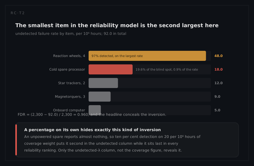
| Cold spare processor | 20 | 10.0% | 18.0 |
| Total | 2,300 | 92.0 |
FDR = (2,300 − 92.0) / 2,300 = 2,208 / 2,300 = 0.960
The 96% is a design target set before anything is built, not a figure measured afterwards, and the reason is the one already given: there is no later. What the undetected column exposes is more interesting than the headline. The cold spare holds 18 of the 92, which is 19.6% of the whole blind spot sitting on 0.9% of the failure rate. The least significant item in the reliability model is the second largest item in the testability model, and only the undetected-λ column reveals it. A percentage on its own conceals exactly this kind of inversion.
The constraint is priced in bits
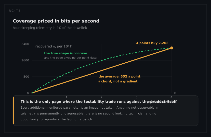
Housekeeping telemetry gets 4% of the downlink. Dividing what that bandwidth buys gives an average exchange rate:
average recovery = 2,208 per 10⁶ h ÷ 4 percentage points = 552 per 10⁶ h per point of downlink
The average is the wrong number to plan the next increment with, and knowing why is the whole discipline. The parameters bought first were the cheap ones: a wheel's speed and current are a handful of bytes a second and light up an enormous share of the wheel population's 1,600 per 10⁶ hours. What remains in the 92 is expensive by construction, because the cheap high-yield monitors have already been taken. Buying the next coverage point means either a high-rate parameter (a bearing vibration spectrum rather than a temperature) or a wide one (full memory maps rather than scrub counts), and both cost bandwidth out of proportion to the λ they recover.
The design response is to move the computation up rather than the data down. A monitor that reduces a spectrum on board and downlinks three summary statistics recovers most of the λ for a fraction of the bits, at the price of committing before launch to which three statistics matter. That commitment is irreversible, and it is the sharpest testability decision on the vehicle.
The wheels give warning, the spare does not
Because the wheels wear, their hazard rises, and the ramp is visible:
h(t) = (β/η)·(t/η)^(β−1)
h(30,660) = (2.2/131,400) × (30,660/131,400)^1.2 = 1.674 × 10⁻⁵ × 0.174 = 2.92 × 10⁻⁶ per hour
h(61,320) = (2.2/131,400) × (61,320/131,400)^1.2 = 1.674 × 10⁻⁵ × 0.401 = 6.71 × 10⁻⁶ per hour
The hazard rate more than doubles from mid-mission to end of mission, and it does so smoothly, driven by bearing lubricant degradation that expresses itself first as rising motor current for the same commanded torque. That is why 97% coverage on the wheels is credible: telemetry is not waiting for a wheel to stop, it is watching a trend that has years to run. The operations consequence is that a wheel can be retired into the spare role before it fails, which is what makes the 3-of-4 architecture worth having.
The cold spare processor offers the opposite case. It accumulates failure through the mission with nothing watching, and the mission is its test interval, so the exposure has to be computed rather than assumed. The rate to use is the flight-lot life rate and not the 200 per 10⁶ hours this page carries as a coverage weight: an exposure is an absolute quantity, and the reliability page is explicit that only the life rates are good for those. Dormant at 10% of the processor's 2 per 10⁶ hours, the spare accrues 0.2 per 10⁶ hours, so
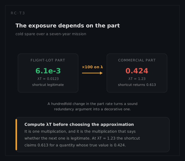
λT = 0.2 × 10⁻⁶ × 61,320 = 0.0123
which is comfortably inside the region where the shortcut is legitimate:
Ulatent = λT / 2 = 6.1 × 10⁻³
The exact form returns 6.107 × 10⁻³ against the shortcut's 6.132 × 10⁻³, a difference of four parts in a thousand that no decision in this analysis can feel. Averaged over the mission the spare is six times in a thousand likely to be dead when it is called, and the recovery path is sound.
That answer depends entirely on the part, and it is worth seeing how fast it stops being true. Build the same spare from a commercial-grade processor of the 200 per 10⁶ hours class and the dormant rate becomes 20 per 10⁶ hours, giving λT = 1.23. The shortcut would then return 0.61, a number not merely inaccurate but on its way to exceeding one, where the exact form gives
U = 1 − (1 − e^(−λT)) / λT = 1 − 0.7067 / 1.2264 = 0.424
Averaged over the mission that spare is 42% likely to be dead already when it is called, and by the end of the seven years the figure is 71%: a credible recovery path in year one and close to a decoration in year seven. A hundredfold change in the part rate turns a sound redundancy argument into a decorative one and simultaneously invalidates the arithmetic used to check it, which is why the exposure product is computed before the approximation is chosen.
Every other system in this chapter resolves that by exercising the dormant item periodically. Here the exercise is a processor switchover on a spacecraft whose purpose is pointing stability, so the test is itself the event the mission is trying to avoid. The design accepts the blind spot and writes the recovery procedure on the assumption that the spare might not answer. What the arithmetic adds is the size of the bet: at flight-lot rates that assumption costs almost nothing, and at commercial rates it is the whole recovery path.
What the analysis tells you to do
Three consequences. First, spend the marginal bit on the wheels' bearing signature rather than on adding breadth, because that is where the trend has years of warning and the recovery action (retire a wheel into the spare role) is available and cheap. Second, treat the 40-minute median time to detect as a budgeted line, not a residual: its mean of 0.85 hours sits inside the 7.35-hour mean restoration that the maintainability page builds from four hours of diagnosis, two and a half of uplink and the detection stage itself, so it is 11.6% of the total, and the availability page shows the imaging clock starting when the fault occurs, not when somebody sees it. Third, schedule a deliberate cold-spare exercise despite the discontinuity, timed into an eclipse or a calibration window where pointing is already interrupted. An annual exercise cuts the exposure from a seven-year interval to a one-year one, λT = 0.2 × 10⁻⁶ × 8,760 = 1.75 × 10⁻³, and λT/2 gives 8.8 × 10⁻⁴, a factor of seven on the only recovery path the computer has. The stronger argument for it is not the factor of seven, which is small against a spare already at six in a thousand. It is that the six in a thousand rests entirely on the dormant rate being what the datasheet claims, and an unexercised spare is the one item aboard that would never contradict it.
What a different technique would have given
The alternative that programmes reach for by habit is to specify and report ground functional test coverage: what fraction of the mode inventory can be detected during integration and test, with the full bench and every connector accessible. That number would be close to 100%, and it would be honest about the facility while describing a capability that ceases to exist at separation. The 4% gap between bench reach and flight reach, 92 per 10⁶ hours of mode inventory, is invisible in the bench figure and permanent in orbit.
The failure mode of that choice is specific: the acceptance campaign passes, the observability requirement is closed against test-facility evidence, and the first anomaly in flight is one whose diagnosis needed a parameter that existed only on the umbilical. On a system with no second look, the only coverage figure worth writing into a requirement is the one computed against the test means that will still be there after launch, which here means telemetry, at 4% of the downlink, and nothing else.