

Two controller boards running active-active, dual hot-swappable power supplies, shelves of drives and a lithium backup unit that holds up the write cache long enough to flush it. The service target is five nines, which is 5.3 minutes of downtime a year, and everything a customer can touch is hot-swappable, so active repair time never enters the availability arithmetic at all. What enters instead is detection and dispatch, which makes this the one system in the chapter where testability is not an input to availability but very nearly the whole of it.
The array also has two test worlds separated by the factory gate. Before shipment the failure population is workmanship (opens, shorts, wrong or misoriented parts, solder voids) and the test access is a structural path through the boards. After shipment it is ageing and drift, and the access is telemetry over a network. Different modes, different instruments, and a single coverage number spanning both would describe neither.
The technique, and why this one
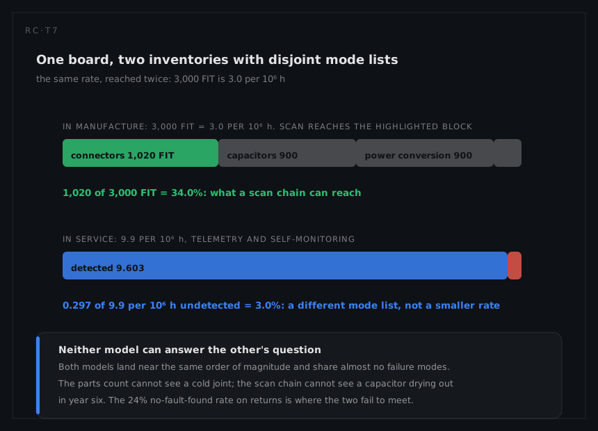
Two dependency models, one per lifecycle phase: boundary-scan structural coverage against the manufacturing defect inventory, and functional telemetry coverage against the in-service failure inventory, each rolled up separately and neither allowed to borrow credit from the other. The split is forced by the mode lists. A scan chain proves that a net is connected; it says nothing about whether an electrolytic capacitor will dry out in year six. A telemetry monitor watches a running board; it never sees the assembly defect that was screened out before the board was ever powered in anger. Merging them yields a headline near 100% that is true at no single moment in the product's life.
| Item | Rate | Model used | Test means |
|---|---|---|---|
| Controller board (each, 2 fitted) | 3,000 FIT = 3.0 per 10⁶ h | constant λ, parts-count prediction | boundary scan in manufacture; telemetry and internal diagnostics in service |
| Power supply (each, 2 fitted) | 1,500 FIT = 1.5 per 10⁶ h | constant λ | output monitoring, fan tachometry, thermal sensing |
| Drive (per drive) | 0.4% AFR = 0.457 per 10⁶ h | renewal process, not a survival question | drive self-monitoring and read-error trending |
| Lithium backup unit | 900 FIT = 0.9 per 10⁶ h | constant λ; protective and demanded only on power loss | continuous state-of-health monitor |
This is the page where a constant failure rate is genuinely correct and should be defended rather than apologised for. The parts are screened, the environment is a temperature-controlled data hall, the equipment runs in its useful life throughout, and the service life is shorter than the onset of any wear-out mechanism in the bill of materials. The drives are the exception on purpose: failed drives are replaced continuously, so the array is designed for a steady arrival of them and the right model is a renewal process.
What boundary scan is actually for
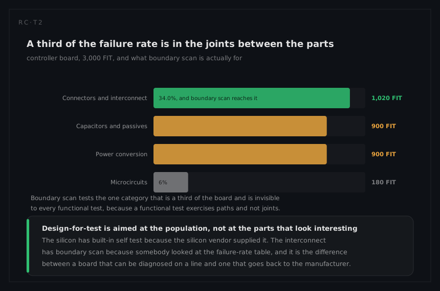
The controller's 3,000 FIT decomposes from the parts count as 180 FIT of microcircuits, 900 FIT of capacitors, 1,020 FIT of connectors and interconnect, and 900 FIT of power conversion. The largest single block is interconnect:
interconnect share = 1,020 / 3,000 = 34.0%
and interconnect is exactly what a scan chain is built to test. Shifting a pattern through every compliant device and observing it at the next boundary detects opens, shorts and misplacements on nets that no functional test reaches reliably, because a marginal joint conducts perfectly well at room temperature on a bench and fails in a hot aisle two years later.
The value of that in the in-service model is indirect and easy to miss. Boundary scan does not raise the 97% telemetry coverage by a single point. What it does is change the population that telemetry has to watch: with assembly escapes screened out, the in-service inventory is a smaller and more tractable set of ageing and drift mechanisms, each with a physical signature something can monitor. Structural test in manufacture is what makes functional coverage in service a question about ageing rather than about workmanship, and a programme that skips it does not get a lower coverage number, it gets the same number computed against a dirtier population.
Rolling up the in-service model
FDR = Σλ(detected) / Σλ(all)
| Item | λ per 10⁶ h | Detected | Undetected λ |
|---|---|---|---|
| Controller boards (2) | 6.0 | 97.0% | 0.180 |
| Power supplies (2) | 3.0 | 98.5% | 0.045 |
| Lithium backup unit | 0.9 | 92.0% | 0.072 |
| Total | 9.9 | 0.297 |
FDR = (9.9 − 0.297) / 9.9 = 9.603 / 9.9 = 0.970
The lithium unit is the worst-covered item, for the reason familiar from every other row: it is protective and dormant, demanded only when mains power fails. It is also the genuine safety hazard in the array, with a thermal runaway failure mode, so its monitor does two jobs at once. Its continuous state-of-health measurement is the third distinct answer this chapter has met to the dormancy question, after the periodic proof test and the partial stroke, and the best of the three where the physics permits it. Checked only at an annual service visit it would carry
Ulatent = λT/2 = 0.9 × 10⁻⁶ × 8,760 / 2 = 3.9 × 10⁻³
whereas a monitor polling cell impedance and charge acceptance continuously collapses T to minutes and the latent term with it. Dormancy is not the problem; unobserved dormancy is the problem, and where an item can be interrogated without being operated, the interval argument disappears entirely.
Detection latency against a 5.3-minute budget
Single-controller unavailability with a four-hour on-site response is the plain product of rate and downtime:
q = λ × MDT = 3.0 × 10⁻⁶ × 4 = 1.2 × 10⁻⁵
and the pair with independent repair gives
q² = (1.2 × 10⁻⁵)² = 1.4 × 10⁻¹⁰
which is why the reliability page concludes the controller pair is not the constraint. The testability qualification is that the four-hour clock starts when the telemetry speaks, not when the board fails. Detection latency adds directly to MDT. With one hour of monitor latency,
q = 3.0 × 10⁻⁶ × 5 = 1.5 × 10⁻⁵
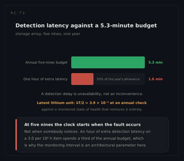
extra unavailable time per year = 3.0 × 10⁻⁶ × 8,760 h = 0.0263 h = 1.6 minutes
Against an annual budget of
(1 − 0.99999) × 8,760 h × 60 = 5.3 minutes
that single hour of latency has spent 30% of the year's allowance. Put the other way, a monitor that takes an hour to notice consumes 60/5.3 = 11.3 years of the annual allowance in one event, if the event is not masked. The 0.18 per 10⁶ hours of undetected controller rate is worse still, because a silent fault in one board turns the q² promise back into a single controller while the dashboard shows green, and nothing starts any clock at all.
The same budget explains the operational rule that looks like a software preference and is actually an availability constraint: 5.3 minutes a year multiplied by four years is 21.2 minutes, so a single disruptive twenty-minute firmware update spends four years of the budget at once, and the availability page shows why rolling non-disruptive updates are not a convenience but the only way the target survives.
What the analysis tells you to do
Instrument for latency, not only for reach. The coverage figure is already 97% and another point is worth less than halving the time to notice on the modes already covered, because latency multiplies straight into MDT for every one of them. Where a monitor is polled, shorten the poll; where it is inferred from a failed operation, add an active probe.
Then confront the honesty measure. Pairing 97% coverage with a 24% returned-unit no-fault-found rate is the sharpest lesson in this row: detection and precision are independent axes. Per thousand arrays in service the controllers produce
6.0 × 10⁻⁶ × 8,760 × 1,000 = 52.6 genuine board failures a year
so the returned stream is 52.6/0.76 = 69.2 boards, of which 16.6 test good. Part of the cause is structural, in the shared backplane and shared firmware build that make symptoms ambiguous across the pair, and part is behavioural: when a hot swap costs no downtime, the fastest route to a closed ticket is to change the board. The cheaper a replacement is, the more the diagnosis has to be right, because nothing else stops the swapping. Tracking the returned-unit rate per symptom code through FRACAS is the only way to tell which half is which.
What a different technique would have given
The alternative in manufacture is to drop the scan chain and rely on end-of-line functional test: power the board, run the product's own diagnostics, ship what passes. It is cheaper, it needs no design-for-test discipline, and it tests the thing the customer will actually use.
What it misses is the 34% of the board's rate that lives in connectors and interconnect, because a functional test exercises a net only if the function it supports happens to run, and a marginal joint passes at benign temperature. Those escapes do not vanish; they arrive in the field as early-life failures indistinguishable from ageing, which pollutes the in-service model's mode inventory and inflates precisely the ambiguous-symptom population that drives the 24% no-fault-found stream. A single lifecycle-wide model fails differently: claiming the union of both layers gives a headline near 100% while the in-service reality is 97%, and the 0.297 per 10⁶ hours in the gap is the population the warranty argument is actually about. Two phases with disjoint mode lists and disjoint instruments need two models.