

Six hundred volumetric infusion pumps in one hospital, each running about 2,500 hours a year, repaired to board level by one biomedical department. The corrective repair takes forty-five minutes, which is nearly the least interesting quantity on this page, because a pump returns to the ward not when the repair finishes but when the department gets to it, finishes it, and someone walks it upstairs.
Every other system in this chapter has one machine and, in effect, one repair. This one has six hundred machines and a single shared service channel, which changes the mathematics. Repair times become service times, failures become an arrival process, and the quantity the wards experience is a waiting time no individual repair time contains. The right instrument is a queue.
The technique, and why this one
A single-channel queueing model of the biomedical department, with a lognormal service time, corrected for service-time variability, and Little's law applied to the full ward-to-bench-to-ward loop. The department is the scarce resource and it is shared, which is exactly the condition under which the systems chapter says single-repair means stop being sufficient.
| Quantity | Model used | Value |
|---|---|---|
| Corrective service time | lognormal, σ = 0.7 | mean 45 min, tmed = 35 min |
| Arrival stream | Poisson, rate from the fleet's maintenance-action rate | 2,640 units a year at the bench |
| Bench queue | M/M/1, corrected to M/G/1 for service variability | ρ = 0.733 |
| Full repair loop | Little's law, L = λW | W = 4.7 calendar days |
| Loaner pool | float sized against the mean number absent | 40 pumps |
| Preventive service | deterministic, capacity removed before queueing | 30 min per pump per year |
The staffing figure everything rests on is a planning assumption, not a specification value: two technicians at 1,500 productive hours each, or 3,000 bench-hours a year. Every result below is sensitive to it, which is itself a finding.
The service time
Take the 45-minute active repair as the mean of a lognormal with the canonical spread:
tmed = 45 / e^(0.7²/2) = 45 / 1.2776 = 35.2 min
M(60) = Φ(ln(60 / 35.2) / 0.7) = Φ(0.761) = 0.777
so a little over three quarters of repairs finish inside the hour, while
t₀.90 = 35.2 × e^(1.282 × 0.7) = 86 min t₀.95 = 35.2 × e^(1.645 × 0.7) = 111 min
One repair in twenty takes nearly two hours. On a single machine that is a footnote; in a queue it is a service-time variance, and variance drives waiting time to first order.
The arrival stream, including the failures that are not failures
Each pump runs at 1,460 per 10⁶ hours over 2,500 operating hours, giving 3.65 maintenance actions per pump-year and, across 600 pumps, 2,190 actions a year: failures, plus the battery exchanges the policy schedules, both of which occupy the bench. The bench sees more again, because 17% of what arrives has nothing wrong with it, mostly setup error reported as device failure. If the 2,190 are the other 83%,
A = 2,190 / 0.83 = 2,640 units a year, of which 450 are healthy
Those 450 each consume the full 45 minutes, produce nothing, and arrive as work orders rather than training requests. The safety analysis reaches the same use-error problem from the other direction, finding it behind about four fifths of the over-infusion hazard.
The queue
Preventive service is scheduled and does not queue, so it comes out of capacity first: 600 pumps × 30 minutes = 300 bench-hours a year, leaving 2,700 hours for corrective work and a capacity of 2,700 / 0.75 = 3,600 jobs a year. Over a 250-day working year,
λ = 2,640 / 250 = 10.56 jobs per day μ = 3,600 / 250 = 14.4 jobs per day
ρ = λ / μ = 0.733
For a single channel with Poisson arrivals,
Lq = ρ² / (1 − ρ) = 0.5378 / 0.2667 = 2.02 jobs waiting
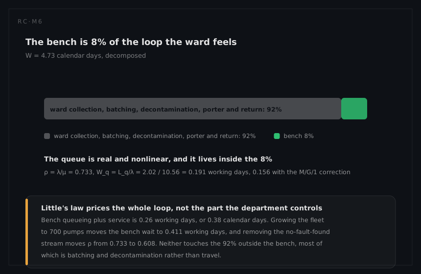
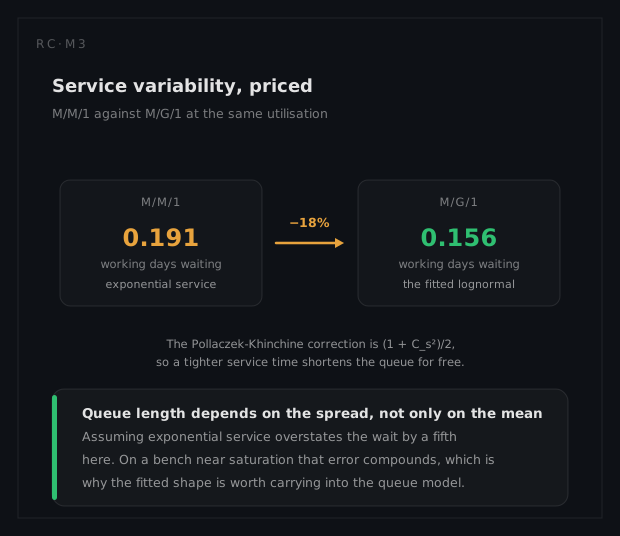
Wq = Lq / λ = 2.02 / 10.56 = 0.191 working days
Service times here are lognormal rather than exponential, and the Pollaczek-Khinchine result scales the wait by the squared coefficient of variation. For σ = 0.7 that is Cs² = e^(0.49) − 1 = 0.632, so
Wq(M/G/1) = Wq(M/M/1) × (1 + Cs²) / 2 = 0.191 × 0.816 = 0.156 working days
an 18% shorter wait than the exponential assumption, because real repair times are less variable than exponential. It cuts the other way in a sloppier workshop: at σ = 1.2 the factor becomes 2.11 and the wait more than doubles, with no change in the mean repair time or the arrival rate.
Three sensitivities make this a queue rather than a sum. They are quoted on the M/M/1 basis, because the variability correction is a constant multiplier and leaves every ratio unchanged.
Arrivals are nonlinear. Strip out the no-fault-found returns and arrivals fall to 8.76 a day, ρ to 0.608 and Wq to 0.108 working days. A 17% reduction in arrivals bought a 44% reduction in waiting; read the other way, the 17% no-fault-found rate is adding 77% to the queue.
Fleet growth is worse than proportional. Take the fleet to 700 pumps and arrivals rise to 12.32 a day, ρ to 0.856 and Wq to 0.411 working days. A 17% larger fleet more than doubles the wait.
Staffing has a cliff, not a slope. Lose one of the two technicians and corrective capacity falls to 1,200 bench-hours, or 6.4 jobs a day, against 10.56 arriving. There is no steady state at all: the backlog grows by 4.16 units a day, about 1,040 pumps a year, until the fleet runs out.
Little's law on the loop the ward feels
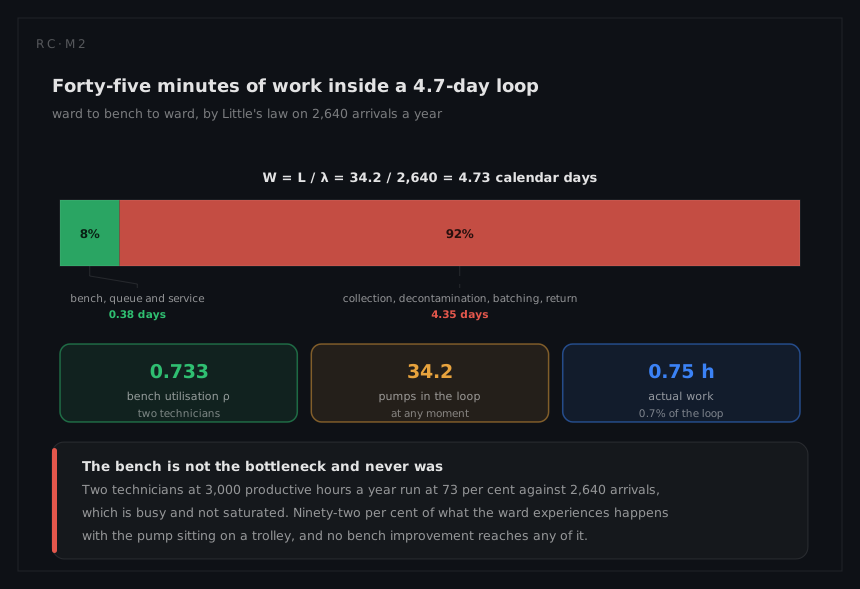
The bench queue is short; the loop is not. Without the loaner pool, fleet availability is 0.943, so the average number of pumps not on a ward is
L = 600 × (1 − 0.943) = 34.2 pumps
and Little's law converts that straight into a turnaround:
W = L / λ = 34.2 / 2,640 years = 4.73 calendar days
The bench portion, queueing plus service, is 0.26 working days or 0.38 calendar days: 8% of the loop. The other 92% is collection from the ward, batching, decontamination, waiting for a porter and the return trip. The closure 1 − 34.2 / 600 = 0.943 reproduces the quoted availability exactly, which is a useful reminder that fleet availability and mean absence are the same statement.
The pool and the permission
The loaner pool is 40 pumps against a mean absence of 34.2, and it delivers exactly what its sizing promises: availability rises from 0.943 to 0.982, leaving a residual 1.8%, or 10.8 pump-equivalents, which is the variance the pool cannot absorb. A float sized at the mean protects against the mean and nothing else, which is why the standard rule adds a multiple of the standard deviation of the number in the system. The availability page works the sizing.
Behind all of it sits a constraint with no arithmetic. The hospital repairs to board level under the manufacturer's service policy, and that policy is why the 45-minute service time exists. Withdraw board-level authorisation and the service time does not change by a second, while the loop becomes a shipment, a queue at a service centre and a return leg, with W in weeks rather than days. That is why the level-of-repair question for medical fleets is settled by service policy and capital budget more often than by technical time.
What the analysis tells the engineer to do
Attack the arrival rate before the service rate. The 450 no-fault-found returns a year are worth 77% of the queue and are fixed by ward training and interface design, not by anything in the workshop. The battery, at 800 of the pump's 1,460 per 10⁶ hours, is the largest genuine contributor and sits on a seven-month cycle at the characteristic life; tightening that interval converts queued work into scheduled work even when total labour is unchanged.
Buy predictability, not speed. The Pollaczek-Khinchine factor says a workshop whose σ drifts from 0.7 to 1.2 doubles its own waiting time while every mean it reports stays constant.
Size the float against the variance. Forty loaners bought 3.9 points of fleet availability. The next few cost far more, and what decides how many to buy is the distribution of L, not its mean.
What a different technique would have given
The technique this replaces is the one most departments actually use: a deterministic capacity calculation. Add the labour, 1,980 corrective hours plus 300 preventive, compare it with 3,000 available hours, and report the department as 76% loaded with 24% headroom. Every number in that sentence is correct.
It is also silent on everything that matters. With constant arrivals and constant service a 76%-loaded server never has anyone waiting, so the calculation predicts a queue of zero, a turnaround equal to the service time, and no benefit at all from reducing the no-fault-found rate. It cannot show that the same department at 86% load waits more than twice as long, and it cannot find the instability cliff: a one-technician department computes as 152% loaded and reports "overloaded", with no way to say the failure mode is an unbounded backlog rather than a longer average. Queues are made by randomness, and a model with no randomness in it has removed the phenomenon it was built to study.