

Two engine-driven integrated drive generators, an auxiliary power unit generator, a ram air turbine, two generator control units and three bus tie contactors, flying five-hour sectors at 3,000 flight hours per aircraft-year. The reliability question asked how often this aeroplane loses all of its alternating-current sources at once. The maintainability question is narrower and more actionable: when a unit fails, what has to happen before the aircraft is serviceable again, and which unit on the list is worth designing for speed.
The second half is where programmes reliably go wrong. The instinct is to attack the longest task time in the maintenance manual, and on this system the longest task belongs to the item that fails least often. The arithmetic that exposes the mistake is one line long, but reaching it means building the task times before any hardware exists to time.
The technique, and why this one
An elemental task-time build-up for each line-replaceable unit, rolled up into a system mean by failure-rate weighting, with a two-branch mixture for the fault-isolation outcome. The choice is forced by where the programme sits in time. The LRU partition, the access routes and the connector counts are decided while the aircraft is still a drawing set, so there is no work-order stream to fit and no fleet whose removals could be measured. What does exist is a design, and a design can be scored element by element against the checklist methods of the maintainability prediction lineage. The weights come from the reliability prediction that produced the item rates.
| Item | Model used for the repair time | Basis | Result |
|---|---|---|---|
| Integrated drive generator | elemental task build-up | pylon access, heavy unit, quick-attach drive pad | 1.5 h |
| Generator control unit | elemental task build-up | rack-mounted, one connector, no adjustment | 0.6 h |
| Bus tie contactor | elemental task build-up | access-dominated, mounted behind structure | 2.2 h |
| System mean corrective time | failure-rate-weighted roll-up | λ from the part-stress prediction | 1.35 h |
| Isolation outcome | two-branch mixture on 88% resolution | testability analysis | 1.38 h effective |
| Downtime at an outstation | additive delay model | 26 h logistics delay on the IDG spare | 27.5 h |
Note what is absent. There is no lognormal, no percentile and no distribution of any kind, because a prediction of this sort produces a mean and nothing else. That is the technique's principal weakness, and the last section returns to it.
Building the times from the task elements
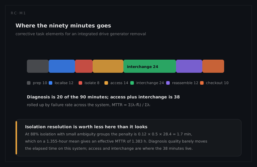
The prediction works through the corrective chain of the foundations chapter, scoring each element against the design feature that governs it. The totals are the specified active repair times; the split across elements is what the prediction produces, and it is the split that tells a designer where to spend.
| Element | IDG (min) | GCU (min) | Contactor (min) |
|---|---|---|---|
| Preparation | 10 | 5 | 12 |
| Fault localization | 12 | 8 | 15 |
| Fault isolation | 8 | 6 | 10 |
| Disassembly and access | 14 | 3 | 45 |
| Interchange | 24 | 6 | 20 |
| Reassembly | 12 | 2 | 20 |
| Alignment and calibration | 0 | 0 | 0 |
| Checkout | 10 | 6 | 10 |
| Total | 90 (1.5 h) | 36 (0.6 h) | 132 (2.2 h) |
Three readings fall straight out. The contactor spends 45 of its 132 minutes, 34% of the job, simply reaching the unit and 20 more putting the structure back: its repair time is not a repair problem but a layout decision taken by someone optimising for weight and routing. The GCU spends 14 of 36 minutes, 39%, on localization and isolation, the signature of an electronics-dense item where diagnosis dominates exchange. And every unit shows zero alignment time, which stored configuration and self-calibration bought back from an element older architectures charged ten to thirty minutes for.
The roll-up, and the offender it names
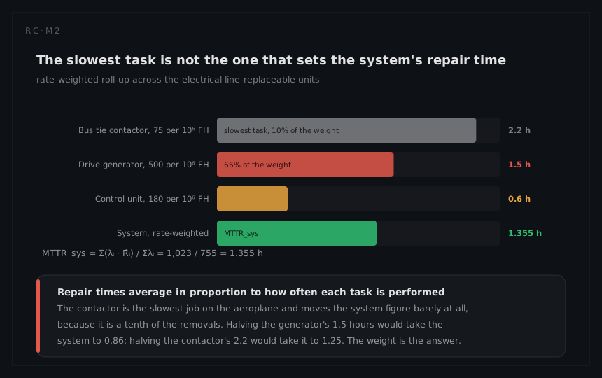
The system mean is the mean over repair events, and events arrive in proportion to failure rates:
MTTRsys = Σ(λᵢ · R̂ᵢ) / Σλᵢ
| Item | λ per 10⁶ FH, all fitted | R̂ᵢ (h) | λᵢ × R̂ᵢ | Share of expected repair hours |
|---|---|---|---|---|
| Integrated drive generator (2) | 500 | 1.5 | 750 | 73% |
| Generator control unit (2) | 180 | 0.6 | 108 | 11% |
| Bus tie contactor (3) | 75 | 2.2 | 165 | 16% |
| Roll-up | 755 | 1,023 | 100% |
MTTRsys = 1,023 / 755 = 1.355 h
Halve the contactor's 2.2 hours, which means moving it out from behind structure and is a serious airframe change, and the weighted total falls to 940.5, giving 940.5 / 755 = 1.246 hours: an 8% improvement. Halve the IDG's 1.5 hours instead and the total falls to 648, giving 0.858 hours, a 37% improvement, because the IDG fails often enough to dominate the event population with a middling task time.
One bookkeeping trap is worth naming while the table is in view. The 755 counts all three contactors, because all three generate maintenance events; the 730 per 10⁶ flight hours quoted as the generation-chain series sum on the reliability page counts only the items in the mission success path. The maintenance population and the mission-reliability population are different lists, and reusing one for the other is among the commonest ways a maintainability prediction goes wrong.
The ambiguity branch, and where its cost lands
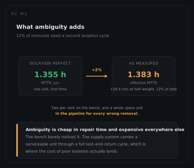
Every time above assumes the technician knows which box is at fault. The testability analysis says that is true 88% of the time. Take the ambiguity group as two units with equal priors, making the expected number of interchange-and-checkout cycles 1.5 rather than 1. The extra half-cycle costs the interchange plus checkout elements, weighted across the event mix:
extra cycle = (500 × 34 + 180 × 12 + 75 × 30) / 755 = 21,410 / 755 = 28.4 min
effective MTTR = 1.355 + 0.12 × (0.5 × 28.4 / 60) = 1.355 + 0.028 = 1.383 h
Twenty-eight minutes of extra work, met on 12% of events at half weight, adds 1.7 minutes to the system mean. At 88% isolation with small ambiguity groups, diagnosis quality barely moves the elapsed time. Where it moves things is the spares ledger. At 755 per 10⁶ flight hours and 3,000 flight hours a year each aircraft generates 755 × 10⁻⁶ × 3,000 = 2.27 events a year on this system, of which 0.27 begin ambiguous, and each of those has an even chance of drawing the wrong unit from a shelf that in the IDG's case holds one spare, at one base. The testability analysis behind the 88% is a maintainability document, but the property it protects is the pipeline, not the clock.
What the numbers tell the engineer to do
Read the labour ledger separately from the elapsed one. At MMH/OH of 0.09 and 3,000 flight hours a year the system consumes 270 maintenance man-hours per aircraft-year. The corrective removals above account for 2.27 × 1.355 = 3.1 elapsed hours, about 9.2 man-hours at three technicians per event, or 3.4% of the labour bill. The rest is scheduled inspection, servicing and troubleshooting that never appears in an MTTR table.
Attack the logistics delay, not the removal. Inherent availability is 0.9991 and operational availability 0.9962, and the entire gap is a 26-hour wait for an IDG spare at an outstation. Total downtime is 27.5 hours, of which the removal is 5.5%. A second spare position, or a different level-of-repair answer, touches all of it; the availability page prices the options.
Recognise what dispatch relief already bought. Permission to fly for up to three days with one IDG inoperative converts the 26-hour wait into no downtime at all, because the aircraft flies home to the spare. The most valuable maintainability feature on this system was bought by the reliability engineer and is certified by the built-in test coverage on the testability page.
What a different technique would have given
The tempting shortcut is to skip the weighting and average the manual's task times: (1.5 + 0.6 + 2.2) / 3 = 1.433 hours, within 6% of the correct 1.355. That closeness is what makes it dangerous, because the number survives review while ranking the contactor first when the contactor is 16% of the problem. Weighting by units fitted is worse, giving (2 × 1.5 + 2 × 0.6 + 3 × 2.2) / 7 = 1.543 hours and the same wrong ranking. An unweighted average is not a rough version of the right answer; it is a different answer to a question nobody asked.
The alternative that genuinely supersedes this analysis arrives later. Once the fleet flies, a lognormal fitted to observed removals replaces the prediction and delivers what the prediction structurally cannot: a spread. At the same 1.355-hour mean and the chapter's canonical σ = 0.7 the median would be 1.355 / e^(0.7²/2) = 1.06 hours and the 95th percentile 1.06 × e^(1.645 × 0.7) = 3.35 hours. A turnaround plan built on 1.35 hours and one built on 3.35 are different plans. The prediction was not wrong; it simply had no way to say that one removal in twenty takes two and a half times the mean.