

One emergency diesel generator, its fuel oil system, starting air, a load sequencer and an output breaker, two trains per unit, demanded only when offsite power is lost. Every other system in this column can be watched: it runs, it stops, and a log records the difference. This machine spends its life not running, and watching it work is itself the thing that makes it unavailable.
Its availability therefore cannot be observed at all in the ordinary sense. The uptime record says the train was available for 8,736 hours last year, and that statement is compatible with the train having been incapable of starting for six months. What replaces the record is a ledger with three lines in it, kept in a currency that is a probability rather than a fraction of time, and the largest line is one that no instrument ever showed.
The technique, and why this one
On-demand unavailability accounting: a three-line standby ledger of test-out-of-service time, latent λT/2 exposure and corrective outage, kept alongside the per-demand failure probability in its own currency and combined in a fault tree with a beta-factor common cause. The technique is forced by the duty. A standby machine has no meaningful uptime ratio, because uptime without a demand proves nothing; the quantity of interest is the probability that a demand arriving at a random instant is answered. That probability has three distinct ways of failing, they have different owners, and two of them are invisible.
| Contributor | Availability model | Parameters |
|---|---|---|
| Surveillance testing | scheduled out-of-service time | monthly start, 2 h out of service each |
| Latent dangerous failure | λT/2 sawtooth, periodically proof tested | λDU = 45 per 10⁶ h; T = 730 h |
| Corrective maintenance | bounded by licence condition | allowed outage time 72 h |
| Failure to start | per-demand binomial, measured | 3.0 × 10⁻³ per demand, from 18 failures in 6,000 demands |
| Failure to run | exponential, over the mission | 1.0 × 10⁻³ per hour, 24-hour mission |
| Fuel oil, starting air, load sequencer | exponential support systems | 250, 180 and 60 per 10⁶ h |
| Two trains | fault tree with β-factor common cause | β = 0.05 |
Three lines, and the one nobody can see
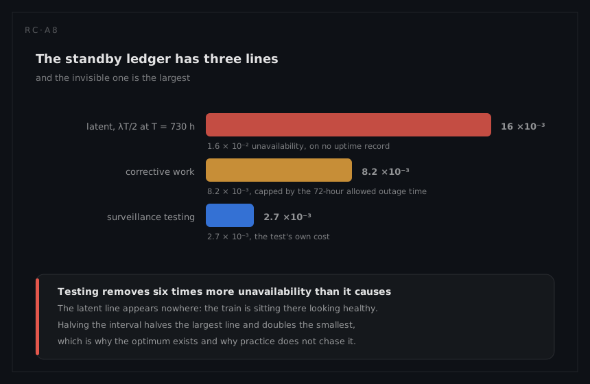
Twelve surveillance starts a year, two hours out of service each:
Qtest = 12 × 2 / 8,760 = 24 / 8,760 = 2.7 × 10⁻³
The train has failed silently since the last test with a probability that climbs linearly between tests and averages half the peak, which is the sawtooth from the foundations chapter:
Qlatent = λDU × T / 2 = 45 × 10⁻⁶ × 730 / 2 = 1.6 × 10⁻²
And corrective work is bounded, not by an engineering estimate, but by a licence condition: the technical specifications allow 72 hours before the plant must shut down. Used once in a year, that is
Qcorrective = 72 / 8,760 = 8.2 × 10⁻³
which is a conservative reading, since the allowance is a limit and not an expectation. Summed with due caution the train sits near 2.7 × 10⁻², and the latent line alone is six times the surveillance line and twice the corrective line. The largest contributor to this machine's unavailability is the one that appears on no dashboard, generates no work order and takes no time.
The three lines are ledger entries to be understood separately rather than added carelessly. The 1.6 × 10⁻² latent term and the 3.0 × 10⁻³ per-demand start failure describe overlapping populations seen through different instruments: some of the failures counted in the surveillance record as failures to start are exactly the dangerous undetected failures the λT/2 term is estimating. Adding them as though independent is one of the classic ways to double-count a standby system's unavailability, and keeping that bookkeeping straight is part of what the fault tree is for.
The test is on both sides of the ledger
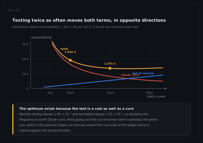
The surveillance start causes 2.7 × 10⁻³ of unavailability and removes 1.6 × 10⁻² of it, and the two move in opposite directions when the interval changes. Halve the interval to 365 hours:
Qlatent = 45 × 10⁻⁶ × 365 / 2 = 8.2 × 10⁻³
Qtest = 24 × 2 / 8,760 = 48 / 8,760 = 5.5 × 10⁻³
combined: 1.92 × 10⁻² falls to 1.37 × 10⁻²
Testing more often is still winning at this interval, which is what the optimum-test-interval argument predicts while the latent line is six times the test line: the marginal gain from halving T is half the latent term, and the marginal cost is only the test term. The optimum is where the two marginal lines cross, and the arithmetic deliberately omits the third effect that will find it. Each start cycle is wear on the machine, so tests eventually begin manufacturing the failures they are looking for, and the crew running them accumulates dose. The testability page works that trade with the numbers; the maintainability page prices the dose constraint that bounds how long any one worker may stay on a job.
The demand-side answer, and the second train
The three-line ledger describes whether the train is there. The per-demand arithmetic describes whether it works, and it is measured rather than predicted, because monthly surveillance across decades produces enough demands to estimate the start probability directly. One train over a 24-hour station blackout mission:
Frun = 1 − e^(−1.0 × 10⁻³ × 24) = 1 − e^(−0.024) = 2.37 × 10⁻²
Ftrain = 3.0 × 10⁻³ + 2.37 × 10⁻² = 2.67 × 10⁻²
Two trains treated as independent would give (2.67 × 10⁻²)² = 7.1 × 10⁻⁴. They are not independent: both share a design, a maintenance organisation, a fuel supply, a set of procedures and an environment. With β = 0.05,
independent part = (0.95 × 2.67 × 10⁻²)² = 6.4 × 10⁻⁴
common-cause part = 0.05 × 2.67 × 10⁻² = 1.3 × 10⁻³
Fpair = 2.0 × 10⁻³
The common-cause term is roughly twice the independent one, which has a direct availability consequence: a third identical diesel attacks the 6.4 × 10⁻⁴ and leaves the 1.3 × 10⁻³ untouched, so difference buys more availability than duplication. The reliability page works the estimation and its confidence bound; the safety page works the consequence, where this unavailability enters a plant-level risk model as a direct input to core damage frequency.
The 72 hours is not a target
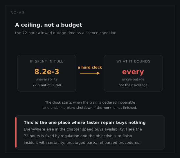
The allowed outage time deserves separate treatment, because it is unlike any other quantity in this column. It is an availability limit imposed as a licence condition: not a budget, not a goal, but a hard clock that starts when the train is declared inoperable and ends in a plant shutdown if the work is not finished. With two trains fitted, taking one out leaves the safety function on a single string, which is why the clock is enforced literally and why corrective work is planned into the refuelling outage wherever it can wait.
It also inverts the usual maintainability argument. Everywhere else in this chapter, faster repair buys availability. Here the 72 hours is fixed by regulation and the engineering objective is not to finish faster but to finish inside it with certainty, which means prestaged parts, rehearsed procedures and rotating crews rather than a shorter task time. A repair that takes 40 hours and a repair that takes 60 hours have the same availability consequence; a repair that takes 80 hours shuts down the unit.
What the analysis tells the engineer to do
The ledger ranks the actions and the ranking is not intuitive. First, attack the latent term, because at 1.6 × 10⁻² it is larger than everything else on the page put together. Shortening the surveillance interval is the direct route and buys 8 × 10⁻³ per halving until wear catches up. Converting latent failures into announced ones is the better route where it is available: any failure that continuous monitoring reveals immediately moves out of the λT/2 regime and into the ordinary announced-failure regime, and it is the only intervention that improves the term without adding starts.
Second, attack β rather than adding hardware. Diverse fuel supplies, staggered maintenance so that one crew never works both trains in the same shift, physical separation and different procedures all reduce the coupling, and once β is admitted it is the only term that scales.
Third, leave the 2.7 × 10⁻³ surveillance line alone. It is the smallest of the three, it is the price of knowing anything at all about this machine, and every attempt to reduce it by testing less makes the largest line worse at six times the rate.
What a different technique would have given
The obvious alternative is the one the availability formula invites: steady-state time availability from the uptime record. The train is out of service 24 hours a year for testing, so
A = (8,760 − 24) / 8,760 = 0.99726
Ninety-nine point seven per cent, and it is a fiction. The honest figure is 1 − 2.7 × 10⁻² = 0.973, ten times worse in unavailability terms, and the entire difference is the latent term the uptime record is structurally incapable of seeing. A time-based availability measure applied to a standby machine measures the diligence of the test programme and nothing else, and it improves whenever testing is reduced, which is precisely backwards.
A second and more tempting alternative is to fold the start failure into a per-hour rate and treat the diesel like any other repairable item, computing an MTBF from the supporting systems (250 plus 180 plus 60 gives 490 per 10⁶ hours, an MTBF of 2,041 hours) and pairing it with a repair time. That model has no per-demand term at all, so it cannot represent the single most likely way this machine fails, which is that it does not start. It would also get the mission-length sensitivity wrong in both directions: a six-hour mission is dominated by the start term and a week-long blackout by the run term, and only a model that keeps the two clocks separate answers both.